
USING MACHINE LEARNING TO PREDICT PRICE DISPERSION
AARON BODOH-CREED, J
¨
ORN BOEHNKE, AND BRENT HICKMAN
Abstract. Theory suggests two sources of price dispersion amongst homogenous goods: market
frictions or product heterogeneity. We collected posted-price listings for Kindle Fire tablets from
eBay to determine if listing heterogeneity can explain the high degree of dispersion we observe. Using
a basic set of controls and empirical techniques in line with the previous literature, we can explain
only 13% of variation in posted prices, which is also in keeping with previous research. However,
we can explain 42% of the dispersion by applying machine learning to a richer set of variables,
which we extract from raw downloaded HTML pages. We interpret this number as a bound on the
role of market frictions in driving price dispersion. Variables describing the amount of information
in the listings, the style of the listings, and the content of the listings’ text are effective price
predictors independently of one another. Our analysis suggests that the content of the listings’ text
plays a primal role in generating the predictions of the machine learning estimator. We repeat our
analysis on a cross-section of products across a variety of categories on eBay, including household
products, sporting goods, and other consumer electronics, and we find a comparable degree of price
predictability across all of the products.
1. Introduction
The “Law of One Price” (LOP) is a prediction from economic theory that all exchanges of
homogeneous goods in a thick, frictionless market ought to take place at a single price. However,
the LOP fails to describe reality in many settings, a fact that was pithily summarized by Hal
Varian, who wrote “the law of one price is no law at all” (Varian 1980 [51]).
In the infancy of online shopping it was thought that the LOP might be more realistic in on-
line markets due to heavy participation by buyers and sellers and database technology that would
seem to make product search as frictionless as possible. To the contrary, however, non-trivial price
dispersion online quickly became a well documented fact, even for products that appear homoge-
neous, such as new books (e.g., Bailey 1998 [6], Brynjolfsson and Smith 2000 [16]). In a model with
rational buyers and sellers, price variation for seemingly homogeneous products can arise from two
sources. First, it could be that units of a given product are actually heterogeneous in subtle ways
that are apparent to consumers, but difficult for researchers to detect in the data. For example,
sellers may bundle complementary objects like accessories or a warranty as means for differentiat-
ing an otherwise homogenous product. Second, market frictions (e.g., search costs or informational
asymmetries) combined with strategic competition between sellers could endogenously generate
Key words and phrases. Online Markets, Price Dispersion, Machine Learning
JEL subject classification: D4, D43, L86
.
1

2 AARON BODOH-CREED, J
¨
ORN BOEHNKE, AND BRENT HICKMAN
equilibrium price dispersion for homogeneous products.
1
Since the various search friction models
imply pricing noise which is plausibly orthogonal to observable characteristics (e.g., mixed pricing
strategies, see Baye, Morgan and Scholten 2006 [11]), any predictive power to be found places a
bound on the role that search frictions could play.
If observable product heterogeneity can explain price dispersion, then in principle it should be
possible to identify features of the product listings that predict the listings’ prices. Our goal is to
maximize the fraction of the price variability that can be explained by product heterogeneity (and
hence need not be explained by market frictions) using richer data in combination with machine
learning methodologies. We analyze a unique and very detailed dataset consisting of posted-price
listings for new Amazon Kindle Fires culled from the eBay marketplace. The dataset includes the
entire HTML code for each listing, so we can observe essentially everything the buyer sees with the
exception of the visual content of the non-stock photos. This provides a rich set of data on which
to estimate our preferred machine learning model, a random forest (Breiman 2001 [15]). These two
contributions, the richer dataset and the use of machine learning, are meant to solve two potential
problems—omitted variable bias and functional form mis-specification—which may have limited
price prediction power in previous empirical studies. Although our empirical model is predictive in
nature, for our purposes we need not identify a causal demand system in order to parse between
product heterogeneity and market frictions as sources of price dispersion.
There are several reasons that we are interested in investigating the magnitude of search fric-
tions on eBay. Market frictions cause waste in terms of user time and effort spent searching, which
could dissuade potential buyers from using the platform. Second, market frictions generated by
strategic competition between sellers result in rents for the firms. Since controlling the balance
of rents received by buyers and sellers is an important strategic decision for competing platforms,
understanding these frictions is a crucial aspect of platform design (Rochet and Tirole 2003 [42]).
In either case, alleviating (or at least controlling) these market frictions is important for platform
service providers. Peer-to-peer platform markets are becoming more prevalent in the online econ-
omy. Examples include Upwork, a platform for recruiting freelance workers; Match.com, a platform
for finding potential romantic partners; and StubHub, a market for buying and selling tickets to
live events. Since eBay is a mature and well established platform, one would expect newer online
markets to exhibit at least the same degree of frictions.
From a theoretical perspective, we are interested in the source of price variation on eBay in
order to test basic models of price formation in perfectly competitive markets. eBay’s posted-price
market for new, first-generation Amazon Kindle Fire tablets, which we refer to simply as “Kindles,”
closely resembles the canonical model of a perfectly competitive marketplace. The eBay market
is quite thick, with thousands of buyers and sellers interacting regularly. In addition, many of
the obvious sources of product heterogeneity are ruled out in our setting. For example, bundling
of new Kindles with accessories is rare in the data, and when present the accessories are of low
value. Seller reliability might induce product heterogeneity, but eBay’s strong warranty against
seller misbehavior should eliminate this as a first-order concern for buyers. These features suggest
1
We discuss the various theories for how market frictions generate price dispersion in Section 2.

PREDICTING PRICE DISPERSION 3
that consumers ought to view the various seller listings as near-perfect substitutes. Yet, we find
that the standard deviation of the price for new Kindles on eBay is 21.2% of the mean price.
2
In order to provide a theoretical benchmark for our analysis, online Appendix B provides a
simple model of a dynamic, frictionless posted-price setting with profit maximizing sellers that
have heterogeneous reservation values (or, alternatively, storage costs). We show that if there is
variation in the day-to-day market clearing price, then all sellers ought to choose a price near the
top of the support of the distribution of market-clearing prices. The intuition is rather simple:
if sellers are patient and the storage costs are not outlandishly large, then patient sellers ought
to be willing to wait for their listing to sell for a high price on a day when the market-clearing
price is idiosyncratically high. However, if all sellers behave in this manner, then there cannot be
nontrivial variation in the market-clearing price. Since price dispersion clearly exists in the real
world, some assumption of our model must be violated. Our analysis focuses on the roles of product
heterogeneity and market frictions in driving price variation, but there are other possibilities that
we do not view as plausible given the features of the eBay platform and the fact that the Kindle is
a small consumer electronics device. For example, the sellers could be impatient or have very high
storage costs, which seems unlikely for a small consumer electronics product. The sellers might not
have rational expectations, but 90 days of prior listings with the sales outcomes are available on
the platform to inform seller expectations. Sellers could also price in a non-profit-maximizing (i.e.,
irrational) fashion or make mistakes, but we feel it is unlikely that this is driving the behavior of
a sizable fraction of the sellers, many of whom have an extensive eBay participation history.
It is worth taking a moment to identify what distinguishes the eBay posted price market for
Kindles from other markets for homogenous products. For example, spot markets for commodities
(e.g., gasoline) exhibit substantial price variation. In reality, these markets contain liquidity traders
that have a need to transact in the near-term that, in effect, renders them “impatient.” For
example, oil refiners pay significant storage costs for their products, which makes them impatient
sellers. While it is easy to imagine time constraints that could make buyers on eBay impatient,
such as the need to purchase a present for a quickly approaching holiday, it is hard to see why
sellers would be eager to be rid of an easy-to-store, relatively inexpensive electronics product when
waiting might bring a significantly higher price.
Our raw data consist of 1,298 downloaded HTML pages listings for new Kindles on eBay. These
pages allow us to see virtually all information displayed to the buyer. The first portion of each
listing’s webpage includes the seller-supplied title and photos of the product, the price and ship-
ping cost, and a measure of the seller’s reputation computed by eBay. The second section is a
standardized description of the product, provided by eBay, that concisely spells out the technical
features of the Amazon Kindle, as well as eBay’s definition of a “new product.” The third section
2
One possible concern is that perhaps many eBay sellers incorrectly list used items as “new,” but this does not appear
to be a meaningful problem in our dataset. A manual inspection of 200 listings revealed 78 listings that explicitly
mentioned that the item was factory sealed, three listings suggesting the box had been opened, and the remaining
listings either had no seller customized description or did not explicitly repeat the definition of a “new” item beyond
what eBay provides as a standard description for new Kindles. We found no examples of items with significant usage
prior to listing the item for sale.

4 AARON BODOH-CREED, J
¨
ORN BOEHNKE, AND BRENT HICKMAN
of each listing displays additional, customizable information provided by the seller and can include
additional photos and/or formatted textual descriptions.
The information contained in the first and third sections is almost entirely at each seller’s dis-
cretion and is highly variable across listings. We captured all text information the seller provided
about the product, as well as the number, size(s), and type (stock or non-stock) of the photos the
seller posted in his or her listing. We find that the item description provided by the sellers varies
widely from listing to listing. For example, the listings had an average of 4.09 photos with a stan-
dard deviation of 4.39. Listings also had an average of 131 words of text written by the seller, but
the standard deviation of the number of words is 280 and 16% of listings include no seller-provided
description at all. We also parse the content of the text using a bag-of-words (BoW) approach,
leaving us with a total of 220 regressors that characterize each of the Kindle listings in our dataset.
Our first goal is to assess the amount of price variation we can explain by applying machine
learning techniques to these high-dimensional observables. The existing literature has made little
headway in explaining online price variation, but we investigate whether this is because previous
studies have ignored some information observed by the user (e.g., our text and image variables),
inducing an omitted variable bias, or whether the cues that consumers extract from these data
manifest themselves in complex and subtle ways that are masked by restrictive functional forms
used in previous studies (e.g., ordinary least squares versus machine learning models), or both.
To address this question, we first construct a restricted dataset using only regressors comparable
to those employed in the prior literature. We measure the independent importance of our richer
dataset by comparing the explanatory power of a given model estimated on the restricted data to
the explanatory power of the same model estimated on the full dataset. The importance of the
model employed is assessed by comparing the predictive power of the two models estimated on the
same dataset. Throughout we measure price predictability using a modified form of the R
2
statistic
that is applicable to both OLS and the random forest algorithm. We can explain 13% of the price
variation using an ordinary least squares (OLS) model and our basic dataset, which is in line with
the weak predictive power observed in the previous literature.
3
An OLS model estimated on our
full set of variables explains 19% of the price variation, meaning the rich set of regressors alone
improves the predictive power of OLS, but only slightly.
We then examine the predictive power of an alternative model based on a random forest (Breiman
2001 [15]).
4
Much like a k-nearest neighbor or a kernel-smoothed regression, a random forest uses
observations that are near the point of interest to generate a localized prediction. A single regression
tree uses a data-driven algorithm to partition the space of regressor values to define what “near the
point of interest” means. Then one level up, a random forest averages the predictions of an ensemble
of regression trees to make a prediction. Random forests have proven popular due to their ability
3
See Section 2 for a brief discussion. This comparison with the previous literature is not intended as a model
selection exercise for many reasons (e.g., the differing datasets). Rather, we wish to make the simpler point that the
vast majority of observed price variation remains unexplained if one relies on OLS techniques and basic observables,
as in the prior literature.
4
We also experimented with other methodologies such as neural networks and boosted gradient trees, but we found
these more complex techniques performed no better than a random forest.
PREDICTING PRICE DISPERSION 5
to capture complex interactions between large sets of regressors in a principled way that allows
for relatively little subjective input from the analyst regarding model selection. When we apply
random forest techniques to the basic dataset, we can explain 20% of the price variation. When we
estimate a random forest model using our full dataset, our explanatory power increases to roughly
42% of the price dispersion. The explained price variation is economically significant at over 10%
of the mean price of a new Kindle. In short, both high-dimensional observables and sophisticated
machine learning techniques are required in tandem to adequately capture the complex process of
information transmission between buyers and sellers that leads to explainable price dispersion.
One possible criticism of our OLS approach is that we may have handicapped standard linear
models by estimating an insufficiently flexible model. To explore this possibility, we build a
dataset that includes a complete set of first-, second-, and third-order interactions of our full set
of regressors, which results in a model with 6,463 variables. After using LASSO (Tibshirani 1996
[50]) to choose our regressors, we find that the linear model still explains only 33% of the variation
in prices. Our conclusion is that while a more flexible linear model can (unsurprisingly) predict
a greater degree of price variation, the model would have to be impractically flexible to begin to
approach the capabilities of machine learning methods.
Another important question is whether our results are somehow contingent on the particular
product or product category we are examining. In Section 5.6, we repeat our analysis on a set of
listings for the Microsoft Surface tablet that we scraped at the same time as the Kindle listings.
We find that we can predict 44% of the price variation across the Surface listings. Section 5.7
analyzes listings for 12 products from across several different product categories, all of which were
scraped in 2018. We can predict between 27% and 67% of the price variation for these 12 products
using machine learning and our rich set of observables. Across these disparate product categories,
our results point to two robust qualitative findings. First, price predictive power using OLS and
the basic, traditional set of observables falls far short of the predictive power of maching learning
and our richer observables. Second, it is the combination of the richer data with the more flexible
methodology that is required to achieve full predictive power, as neither suffices on its own. The
fraction of price variation we explain is economically significant since the standard deviation of the
listings’ prices is between 15% and 63% of the mean price. In short, high price predictability seems
to be common on eBay so long as sufficiently rich data are available and flexible predictors are
used.
One common drawback of machine learning is that with its impressive flexibility comes greater
difficulty in interpreting results. In order to better understand the sources of the predictive power
we uncovered, we partition our variables into intuitive subsets that are likely to measure the amount
of information conveyed (e.g., the volume of text and number of images), variables that represent
the style of the listing (e.g., text style and formatting), and BoW variables that describe the
meaning of the listings’ text. In order to pin down which combinations of variables are providing
the predictive power, we analyze the effect of adding different groups of variables to our basic dataset
and deleting different sets of variables from our full dataset. We find that we can generate accurate
price prediction models using each subset of our data, which implies that the different subsets
6 AARON BODOH-CREED, J
¨
ORN BOEHNKE, AND BRENT HICKMAN
contain redundant information. We use a variable importance test to assess which variables are
used most heavily by our random forest, and we find that the BoW variables are most important.
It is easy to come up with an information-based explanation for how the volume of information
or the content of a listing’s text predicts a higher or lower price (e.g., explaining a defect in
the packaging), and these communications are credible because of the incentive sellers have to
maintain good reputations (Cabral and Horta¸csu 2010 [18]). We find that we lose only a small
amount of predictive power by estimating our model on only the basic dataset plus the variables
that summarize the volume of information conveyed. We also find that the style variables (e.g., the
number of HTML tags used in a listing) have as much explanatory power as the variables describing
the volume of the information conveyed by the listing. The style of a listing can convey powerfully
to a potential buyer that the seller is a professional—the design of such a listing is costly, but
professional sellers can defray this cost by repeatedly using the same listing template. We argue
in Section 4.3 that inexperienced sellers cannot simply copy another seller’s stylized listing that
has been tuned to increase the sale price without paying a substantial cost in terms of effort. The
combination of these effects makes the style of a listing a credible signal of professionalism.
At the end of the day, however, we find that significant unexplained price variation persists,
suggesting that search frictions also play an economically meaningful role. This may seem counter
to expectations, given the cutting edge search algorithms at eBay users’ disposal, but one possible
explanation is an “embarrassment of riches” problem. Given the sheer scope of the marketplace, it
may be that there are so many relevant results for a keyword search on the phrase “Amazon Kindle
Fire” that it is still costly for consumers to sift through all of them.
The remainder of this paper has the following structure. We start with a discussion of the related
literature in Section 2. Section 3 provides a description of the mechanics of the eBay posted-price
market and describes the listings that we study. Section 4 describes the data we collected. Section 5
presents basic results on the importance of (i) the richness of our dataset and (ii) flexible estimation
techniques for price prediction, discusses robustness checks, and assesses generalizability. Section
6 explores the underlying structure of the data that is captured by our random forest models. We
conclude and discuss some plausible interpretations of the remaining price dispersion in Section
7. Appendix A provides robustness checks to eliminate various alternative interpretations for our
results. Appendix B provides a model of seller behavior in this market, which we include to highlight
the assumptions required for price dispersion to vanish.
2. Related Literature
Lewis (2011 [34]) conducts an exercise similar to ours in that he examines whether the presence
of phrases associated with vehicle quality (e.g., “dent”) influence the final price received in an
eBay Motors vehicle auction. The goal of the analysis is to assess whether these phrases alleviate
adverse selection, which the results support. Our study and Lewis (2011 [34]) share the goal of
assessing the informational content of the listings. However, Lewis (2011 [34]) focuses on explaining
price dispersion amongst heterogeneous products, whereas we focus on predicting price dispersion
PREDICTING PRICE DISPERSION 7
between putatively homogenous products. In addition, we use a much larger set of observables and
apply machine learning techniques to generate our price predictions.
Price dispersion as a consequence of ignorance has been recognized at least since Stigler (1961
[49]). Building on Stigler’s original model of costly search, Diamond (1971 [21]) proved that
profit maximizing firms can act as monopolists if consumers face search costs. Although the
model of Diamond (1971 [21]) does not yield equilibrium price dispersion, it does show that large
deviations from the perfectly competitive outcome are possible if consumers face small search costs.
Reinganum (1979 [41]) shows that price dispersion can arise when consumers discover prices through
a process of sequential search and firms have heterogeneous marginal costs. MacMinn (1980 [35])
shows that price dispersion can also arise under this market structure when fixed-sample search is
used. The core insight of all of these models is that the search cost enables firms to price above
marginal cost, an effect which is then amplified through strategic interaction amongst the firms.
The price dispersion is generated by the mixed strategies firms use when setting prices.
A second potential source of price dispersion is information asymmetries amongst consumers.
These models assume that firms are homogenous, but buyers are asymmetrically informed either
because of heterogeneous buyer search costs (e.g., Salop and Stiglitz 1977 [45], Rosenthal 1980
[43], Wilde and Schwartz 1979 [53], Varian 1980 [51]) or because of heterogeneous outcomes of a
stochastic search process (e.g., Burdett and Judd 1983 [17]). The firms respond to the asymmet-
rically informed consumers by playing a mixed pricing strategy that generates equilibrium price
dispersion. The more recent literature has applied models of this form to study online price clear-
inghouses as important strategic actors in the affected markets (e.g., Baye and Morgan 2001 [8],
Baye et al. 2006 [11]). We do not believe that these models provide a realistic description of eBay,
with its many participants connected by a common online platform, since they assume sellers have
a captive market of buyers that are either uninformed about the prices of competitors (e.g., Salop
and Stiglitz 1997 [45], Rosenthal 1980 [43], Wilde and Schwartz 1979 [53], Varian 1980 [51]) or are
loyal customers of the firm (Baye and Morgan 2001 [8]).
Although eBay’s web-based, interactive search services would seem, at first glance, to make it
easy to obtain a price quote, it may be costly for the user to parse the search results if the listings
are heterogeneous. The existence of search frictions on eBay has been established in the various
auction markets that eBay runs. Bodoh-Creed, Boehnke, and Hickman (2017 [14]) estimate that
bidders in eBay auctions have a participation cost of $0.07 per bid placed. Backus, Podlow, and
Schneider (2014 [5]) and Schneider (2016 [46]) explicitly test for search frictions by exploiting the
algorithm eBay uses to order the listings served to buyers. As both use a similar methodology, we
discuss the earlier of these papers here. The authors analyze a sample of new DVDs for sale on
eBay and show that including the word “new” in the title of the listing makes it more visible, as
these listings are seen both by buyers that search for the DVD’s title (e.g., “Batman Begins”) and
those that explicitly search for the item (i.e., “Batman Begins new”). The increased visibility of
adding the word “new” results in a 3.5% higher probability of sale and an $0.83 higher sale price
conditional on sale. We argue in Section A.2 that this sort of manipulation of the search algorithm
is not driving our empirical results.
8 AARON BODOH-CREED, J
¨
ORN BOEHNKE, AND BRENT HICKMAN
A large branch of the more recent empirical literature on price dispersion has focused on tests
of various models. For example, Sorenson (2000 [48]) shows that pharmaceutical products that
necessitate repeated purchases have lower price variation since the consumers have a strong incen-
tive to find a low price. Baye, Morgan, and Scholten (2004 [9]) and (2004 [10]) use data from a
price comparison web site and data on the market structure across different products to test the
implications of information clearinghouse models. Baylis and Perloff (2002 [13]) find a combina-
tion of high-quality, low-priced firms competing with low-quality, high-priced firms in the online
markets for scanners and digital cameras, which the authors interpret as support for the two-price
equilibrium predicted by Salop and Stiglitz (1977 [45]). Some papers estimate a structural model
to tease apart the sources of price variation (e.g., Hong and Shum 2006 [30]).
There are prior studies that attempt to predict product prices and report statistics that describe
their explanatory power, but many of the estimates have features that make them difficult to com-
pare with our results. Among the papers that are comparable to our project, Baye, Morgan, and
Scholten (2006 [12]) attempts to predict the price dispersion for online consumer electronics sales.
Their price regression can explain 17% of variation using regressors capturing attributes of the re-
tailers, but the explanatory power jumps to 72% when the regressions include firm-specific dummy
variables. Clay, Krishnan, and Wolfe (2001 [19]) attempts to predict prices and achieves a high
degree of explanatory power, but their regressions include time dummies. Time dummies explain
a great deal of the price variation across our sample due to product depreciation, but this price
variation is unrelated to the cross-sectional price dispersion generated by product heterogeneity.
Clay, Krishnan, and Wolfe (2002 [20]) provides an analysis of the price dispersion of text books
that explains 2.7% of the dispersion when regressions do not include store-level dummy variables
and 19.2% of the dispersion when the dummy variables are included. Pan, Ratchford, and Shankar
(2002 [38]) study the price dispersion across eight categories of retail products and can explain at
most 22% of the price dispersion, with the notable exception being that their regressions explain
43% of price variation for compact discs. Our general conclusion from the empirical literature is
that price dispersion is difficult to explain without including regressors such as seller-specific fixed
effects. Ancarani and Shankar (2004 [1]) find that internet retailers of books and compact discs have
lower price dispersions relative to traditional retailers. Ratchford, Pan, and Shankar (2003 [40])
use BizRate.com data covering a wide array of products to argue that price dispersion decreased
between 2000 and 2001, which the authors attribute to the market maturing.
Since price dispersion results from pricing strategy, the literature on online price setting and
competition is relevant. Lal and Sarvary (1999 [32]) challenged the assumption that internet com-
petition will lead to lower prices, and they formulate a model of how the internet can decrease price
competition. Lynch and Ariely (2000 [33]) find in an experiment that lowering the cost of infor-
mation reduced price sensitivity for differentiated products like wines. Shankar and Bolton (2004
[47]) find that attributes of competition explain most of the variance in retailer pricing strategies.
Even when seller dummy variables can explain a great deal of the price variation, it is unclear
what exactly the dummy variables are capturing. For example, suppose that one concludes that
Best Buy, a brick and mortar electronics retailer in the United States that also has an online store,
PREDICTING PRICE DISPERSION 9
has consistently higher prices than other electronics retailers. The higher prices at Best Buy could
be because the products are different (product heterogeneity), it could be that Best Buy offers
generous return policies (heterogeneous retailers), or that Best Buy has a near monopoly over brick
and mortar electronics sales in many regions that allows the firm to charge higher prices (market
competition).
One of the themes that emerge from our empirical results is that a variety of characteristics
of a listing’s style (e.g., the number of HTML tags used) can serve as signals of a seller’s profes-
sionalism. Elfenbein, Fisman, and McManus (2012 [26]) explicitly study whether assigning part
of an auction’s revenue to a charitable cause can act as a substitute for a high seller reputation.
Although thematically similar to our result, the study used quasi-experimental variation between
listings from the same seller to identify the effects.
Dinerstein et al. (2017 [22]) directly examines a redesign of the eBay platform meant to encourage
buyers to consider low-priced products and enhance price competition amongst sellers. Prior to
May 19, 2011, eBay showed buyers that searched for a product a list of “Best Match” results that
did not explicitly consider price when ordering the products displayed to the user. From May 2011
through the summer of 2012, eBay displayed the posted-price listings in order of increasing total
price. Starting in late 2012 (prior to our data collection period), eBay returned to using the “Best
Match” as the default. Dinerstein et al. (2017 [22]) estimate a model of consumer demand and
assume that users consider a random number of listings that are randomly selected based on either
the listing’s quality or the price under the redesigned platform. They show that price dispersion
decreases when the platform emphasizes low prices.
We would also like to highlight a handful of other papers that have worked directly with eBay
“Buy It Now” data. For example, Hui et al. (2016 [31]) studies the interaction between the effects of
reputational mechanisms and insurance against seller misbehavior on the prices received by sellers
in Buy It Now and auction listings on eBay. Saeedi and Sundaresan (2016 [44]) study a sample of
Buy It Now and auction listings on eBay to understand the effect of a change in the reputation
system on buyer and seller behavior. Other papers have studied the relationship between Buy It
Now postings and auctions with a particular focus on the economic forces that allow the two sales
mechanisms to coexist on the same platform (e.g., Einav et al. 2013 [23], Einav et al. 2016 [24],
Einav et al. 2015 [25]). Nosko and Tadelis (2015 [37]) documents that buyers’ experiences with
sellers spills over onto other sellers, and the authors propose a novel and more effective metric of
interaction quality. Elfenbein, Fisman, and McManus (2015 [27]) study the interaction of the value
of quality certification and market structure. To the best of our knowledge, we are the first to
use data from a platform like eBay to study price dispersion, utilize contextual data (e.g., text or
images) as rich as ours, or bring machine learning techniques to bear to explain price dispersion.
3. The eBay Setting
eBay uses a fine-grained, hierarchical product classification system for the goods listed for sale on
the platform. For example, all Kindles are in the “Tablets & eBook Readers” category, but there
also exists a separate category at the bottom of the hierarchy for new, first-generation Amazon

10 AARON BODOH-CREED, J
¨
ORN BOEHNKE, AND BRENT HICKMAN
Kindle fire tablets with 8 GB of storage. The classification system allows for heterogeneity within
broad product categories (e.g., tablet computers) and very limited product heterogeneity at the
narrowest level of classification.
We focus on the “Buy It Now” listings that use a posted-price format, which make up more than
half of all listings on eBay today. A seller using a posted-price format has the option to provide
title text and a photo that will appear in the page of search results observed by prospective buyers.
For consumer electronics products, the seller must also provide the exact specifications (e.g., 8 GB
of storage) and condition (e.g., “New”) of the product so that it can be placed within the eBay
product hierarchy. The price of the product as well as the shipping options must also be chosen.
The seller can either offer flat-rate shipping or choose to have shipping calculated by eBay. If the
shipping is calculated by eBay, a forecasted price for shipping is computed for a prospective buyer
based on the seller’s and the prospective buyer’s locations as well as package size, weight estimate,
and shipping company specified by the seller. Finally, the seller is allowed to choose the duration
of the listing from a discrete set of options (e.g., 3 days, 7 days, etc.).
In addition to supplying a platform for hosting posted-price listings, eBay provides payment
and sales infrastructure for the buyers and sellers. eBay also provides a money-back guarantee for
buyers, which can be triggered easily through the website and results in a rapid (less than five
days) refund of the money paid to the seller.
A buyer on the eBay site begins by searching for items using keywords and an optional selection of
which broad product category to search within. The user is then served a page of results. Although
eBay continuously experiments with how to order the items on the search page, conversations with
eBay employees during the time our data was collected (28 December 2012 - 20 September 2013)
indicated that items appeared early in the list of results based on (1) whether the listing’s title
included all of the keywords that the buyer included in his query and (2) the timing of the listing’s
termination, with listings that expire in the near future being closer to the top of the search results.
5
After the search results are generated, a buyer can click on a listing on the search results page to
see the webpage for a listing, reorder the search results by price, or view successive pages of search
results. Buying an item requires viewing the webpage for a listing, clicking a “Buy It Now” button
at the top of the listing webpage, and entering the required payment information.
The webpage for a listing that a potential buyer sees once he or she clicks on an item in the search
results page has a format with three sections. Figure 1 displays an example of the first section of
the listing, which we refer to as the title section. The title section includes a brief text description
of the item written by the seller and one or more photos that are provided by the seller. The
title section also has a standardized format that includes the price chosen by the seller, shipping
information, the item’s condition (e.g.,“New”), and a seller reputation score. The seller reputation
score is equal to the total number of positive buyer ratings minus the number of negative ratings.
The second section of each listing is a box that provides a standardized, uniformly formatted set
of information about the product that is provided by eBay, an example of which is depicted in Figure
5
We argue in Appendix A.2 that our results are not driven by the efforts of sellers to manipulate the prominence of
their listing in the search results through choice of the listing’s title.

PREDICTING PRICE DISPERSION 11
Figure 1. eBay’s Standardized Listing Information
2. The box describes the precise definition of the condition of the product and detailed technical
specifications of the product (e.g., CPU processor speed). Since the section is standardized across
our sample, it does not play a role in our analysis. However, the existence of this section shows
that there can be little ambiguity about either the product being sold or the product’s condition.
A fairly elaborate example of the third section of each listing, which we refer to as the description
section, is provided in Figure 3. This third section is created entirely by the seller and is optional,
with about 16% of listings in our sample having no content in the description. The seller has
the ability to provide a large amount of text and images, and the text can be formatted using
HTML tags (e.g., bolded text). The challenge for analyzing the information in the description is
condensing the many features of the text and images into data amenable to statistical analysis.
4. Data
Each data point is a single listing for a new, first-generation Amazon Kindle Fire. We collected
our posted-price listings using a scraping program that captured the listings from sellers located
within the United States that posted to the platform between December 28, 2012 and September
30, 2013.
6
Since our primary interest is the price setting behavior of sellers, we include listings in
our sample regardless of whether they resulted in a sale. We include only listings offering a single
unit, and we eliminated a small number of listings with implausible prices (i.e., below $15), which
yielded a total sample of I = 1, 298 listings. If a seller offered multiple listings across our sample, we
6
We searched in the “iPads, Tablets, and eBook Readers” category using the keywords “Amazon Fire.” This returned
all of the active listings that included either of these words. We did not include the word “Kindle” because this tended
to return listings for much older black and white Kindle e-readers, which were more numerous on the eBay site at the
time. After experimenting with various keyword combinations for our scraping algorithm, we found that the search
phrase “Amazon Fire” provided the best balance of specificity and breadth. This combination of search terms and
keywords allowed us to capture virtually all listings of Kindle Fire tablets on eBay during our sample period.
12 AARON BODOH-CREED, J
¨
ORN BOEHNKE, AND BRENT HICKMAN
Figure 2. eBay’s Standardized Description
treat each listing as a distinct data point. There are 911 unique sellers in our dataset, 5 of which
have 10 or more listings. The vast majority of sellers had very few listings: 79.5% of them had
a single listing and another 12.7% had 2 listings. As a robustness check we analyze the behavior
of sellers that offered multiple listings in Appendix A.3, where we argue that our main results are
invariant to inclusion of these listings.
One concern is that despite the items being listed as in “New” condition, the Kindles might
actually be used and in “Like New” condition. eBay requires that the seller confirm that his or her
product matches the eBay definition of a “New” product before posting the listing, so a mistake by
the seller is unlikely. A manual inspection of 200 listings revealed 78 that explicitly mentioned that
the item was factory sealed. Only three listings indicated that the Kindle had ever been opened
and included comments like “We opened the box and charged the unit & confirmed that it power
[sic] up ok.” Most of the remaining listings either had no description or did not explicitly repeat
the definition of a “New” item that eBay provides above the description. We found no examples

PREDICTING PRICE DISPERSION 13
Figure 3. Seller’s Customized Description
0 5 10 15 20 25
Units Available
120
140
160
180
200
220
Price
Unit Available
Unit Sold
Figure 4. Supply Curve on 23 June 2013
of items with significant usage prior to listing the item for sale, and eBay provides substantial
incentives for sellers not to blatantly lie in their descriptions.
The median day in our sample period had just over two dozen active Kindle Fire listings. An
exemplar of a daily supply curve is shown in Figure 4. On a typical day the listings that result in
sales have lower than average prices, but there are usually higher priced listings that also generate
sales, even when some listings with lower prices go unsold. Some listings exceed the retail price of
14 AARON BODOH-CREED, J
¨
ORN BOEHNKE, AND BRENT HICKMAN
50 100 150 200 250
Days from Jan 1 2013
100
110
120
130
140
150
160
170
180
190
200
Dollars
Figure 5. Price Trend Over Time
$159 on Amazon’s website, but are less likely to result in a sale. It is well documented that eBay
users sometimes pay more than fixed retail prices for goods, so it is not obvious that these high
price quotes are not optimal for sellers. For example, Malmendier and Lee (2011 [36]) find that
more than 40% of auctions exceed the simultaneous fixed price across a broad variety of products,
with overpayment averaging roughly 10% of retail price.
We describe our dataset in three sections. First, Section 4.1 outlines the features of listings that
we collected, and Section 4.2 elaborates on how we incorporate the text data into our analysis.
Section 4.3 closes with a discussion of the features of the eBay market and interface that make
features of the listings credible signals about the product and the seller in equilibrium.
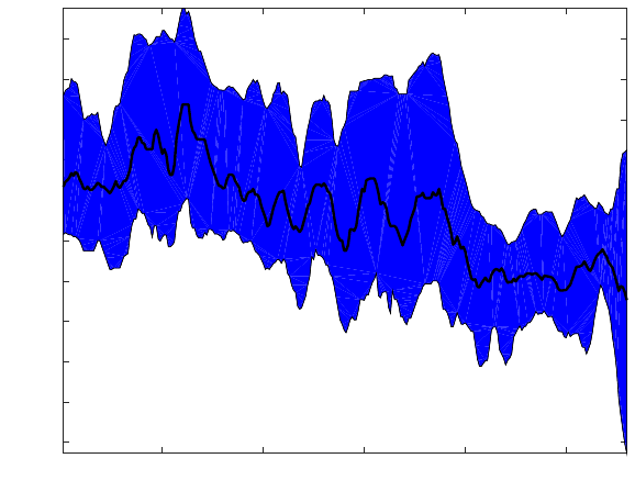
4.1. Variables. Figure 5 provides a time series plot of the median price of the listings on each
day, and the band describes the interquartile range of the distribution of prices. All of the time
series have been smoothed using a seven-day moving average filter. Two features are of note in
Figure 5. First, the market shows no sign of converging toward satisfaction of the LOP by the
end of our nine month sampling period. The persistence of price dispersion is well documented in
other online markets, so this is not terribly surprising. The second feature to note in Figure 5 is
the trend toward lower prices as the sample period persists. Again, this is not surprising since
the value of electronics products depreciates (even new ones) as the anticipated release dates of a
newer version approaches.
It is worth taking a moment to consider the ideal dataset for our purposes and how this informs
our handling of the time trend in our analysis. The ideal dataset would be a snapshot of the prices
offered in a market with hundreds of active listings, which would allow us to hold all time-varying
features of the market fixed and isolate what caused the seller to believe that an unusually high or

PREDICTING PRICE DISPERSION 15
Variable Mean Median Standard Deviation
Price 0 -$1.74 $30.23
Shipping Price $3.71 0 $4.96
Shipping Calculated 0.437 0 0.496
Returns Allowed 0.303 0 0.460
log(Seller Score) 4.78 4.72 2.02
Re-listed 0.168 0 0.374
Table 1. Basic Data Set Summary Statistics
low price was warranted for that listing at that point in time. In other words, we want to explain
price-variation in a cross-section of listings and not across time. Unfortunately, the market does
not contain hundreds of listings on any given day, so we collect listings across days. If we were
to include time dummies or a time trend in our regressions, then we would be able to explain
some price variation simply through these time-dependent variables. However, since our research
focus is on cross-sectional price variation rather than variation over time, the appropriate course
is to de-trend our price variables. Once de-trended using a linear time trend in price, the standard
deviation of the detrended prices is $30.23, which is equal to 21.2% of the raw mean price.
7
For our Basic Data Set we only include variables that are analogous to observables used in earlier
papers that attempted to explain online price variation. Price is either the price at sale or, for
items that did not ultimately sell, the final price the seller offered before removing the unsold item
from the site. Shipping Price is the price of shipping if a flat rate was included in the listing and 0
otherwise. Shipping Calculated is a dummy variable equal to 1 if eBay automatically calculates the
shipping. Returns Allowed is a dummy variable equal to 1 if the seller accepts returns. Re-listed is
a dummy variable set to 1 if the seller chose to re-list the item after the item did not sell during the
listing’s initial duration. Seller Score is a numeric value indicating the net positive feedback left by
individuals that had purchased from this seller previously. Prior work has shown that this statistic
is not perfectly informative of seller quality (see, for example, Nosko and Tadelis 2015 [37]), which
leaves room for the seller to use other aspects of the listing (e.g., layout and content) to signal his
or her professionalism and reliability. In our empirical exercise we will explicitly control for both
sources of information about the seller’s professionalism. Variable names and summary statistics
for the basic dataset are included in Table 1.
Our Full Data Set includes all of the information in the basic dataset as well as features gathered
from the portions of the listing that can be customized by the sellers. These data include the
number of characters, words, special characters, and fraction of upper case characters in the title
and the description of the listing. We record the number and size of the photos provided by the seller
7
We also experimented with higher-order polynomials and did not find any statistically or practically significant
differences from the linear trend model.

16 AARON BODOH-CREED, J
¨
ORN BOEHNKE, AND BRENT HICKMAN
as well as whether the seller used one or more stock images. A stock image is a professional image
of the item that one can download from the internet (e.g., from Amazon’s website), as opposed to
a non-stock image that the seller might take with his or her own camera of the actual item they
are selling. We also capture the number of HTML tags (e.g., sections of bold text), the number of
font sizes, and the number of changes in font size in the seller’s description of the product. These
variables all reflect techniques that a seller might use to make text eye-catching. We also record a
categorical variable describing whether the listing started on the weekend (Saturday or Sunday),
early in the week (Monday - Wednesday), or late in the week (Thursday or Friday). Finally,
we record whether the listing was generated by eBay’s mobile phone app. Summary statistics are
provided in Table 2.
4.2. Natural Language Data. The natural language data was handled using a Bag of Words
(BoW) approach (Gentzkow, Kelly, and Taddy 2017 [29]). First we separated each listing’s text
into sentences and words, and each word was stemmed using Porter’s Stemming Algorithm (Porter
1980 [39]). The stemming algorithm is capable of identifying different forms of the same word. For
example, the stemmer can identify “charges,” “charged,” and “charging” as sharing the same root
“charg.” Correctly stemming the text removes redundant features and insures an accurate count
of the number of appearances of each word. We do not attempt to identify negations (e.g., “no
returns”) algorithmically as this is much more computationally difficult and subject to a greater
error rate. After the stems have been identified and the number of occurrences of each stem in
each listing has been computed, we reduced the dimensionality of the natural language data in
two steps. First, we formed a list of the 1,000 most frequently appearing elements of the BoW.
After eliminating articles and prepositions, we manually reduced the set to 190 word stems that we
thought represent potential sources of heterogeneity and appear in at least 5 of the listings. For a
full list of the words, please see Appendix D.
8
Second, we used principal component analysis (PCA) to further reduce the dimensionality of the
BoW data.
9
PCA is a methodology for projecting a set of data points onto a set of orthogonal
basis vectors, usually referred to as components. To fix ideas, each BoW datum is a 190-dimensional
vector, call it w
i
= [w
1,i
, . . . , w
190,i
]
|
, where w
k,i
indicates the number of times the k
th
word stem
occurred in the seller’s description in the i
th
listing page, minus the mean count of the k
th
word
stem across all listings. The first principal component is chosen by picking a vector of weights or
factor loadings, call it π
1
= [π
1,1
, . . . , π
1,190
]
|
, to construct a linear combination of the regressors,
P C
1,i
= w
|
i
π
1
, that has the highest possible variance subject to the constraint that π
1
has unit
length. The second and following components, each represented by their own factor loading vector
π
j
, j ≥ 2, are constructed to be orthogonal to all previous components, and to have the highest
possible variance subject to the same unit length constraint.
8
We also experimented with using dummy variables for the appearance of a word in a listing as opposed to the word
count. We found it had no effect on our results.
9
We experimented with using the BoW entries as regressors directly but found that this did not result in improved
predictive performance in the random forest model. However, using the BoW counts as regressors in our OLS model
resulted in massive overfitting that caused the OLS out-sample-R
2
(see Section 5.2) to be negative.

PREDICTING PRICE DISPERSION 17
Variable Groups
Variable Mean Median
Standard
Deviation
Title
Length
Number of
Characters in Title
60.1 66 16.4
Number of
Words in Title
10.6 12 2.68
Title
Style
Number of Special
Characters in Title
15.0 16 4.63
% Uppercase
Characters in Title
0.312 0.263 0.168
Title
Images
Number of Photos
in Title
2.15 1 1.86
Number of Stock
Photos in Title
0.439 0 0.509
Description
Length
Number of Words
in Description
131 27 281
Description
Style
% Uppercase Characters
in Description
0.122 0.075 0.184
Number of HTML
Tags in Description
102 16 201
Number of
Font Sizes
1.58 1 1.451
Number of Font
Size Changes
4.33 0 16.0
Description
Images
Kilobytes of Photos
in Description
16.0 0 80.1
Dummy: 1 to 5
Photos in Description
0.103 0 0.304
Dummy: 5 or more
Photos in Description
0.063 0 0.243
Miscellaneous
Variables
Dummy: Posted During
Weekend
0.277 0 0.448
Dummy: Posted During
Early Week
0.429 0 0.495
Dummy: Posted During
Late Week
0.294 0 0.456
Dummy: Posted with
eBay Mobile
0.242 0 0.428
Table 2. Full Data Set Summary Statistics (without Bag of Words data)

18 AARON BODOH-CREED, J
¨
ORN BOEHNKE, AND BRENT HICKMAN
Component Name
% Variance
Explained
Words with
High Loadings
Description of Item 43.6 “new,” “read,” “include,” “content”
Shipping and Payment
Information
11.9 ”paypal,“ ”return,“ ”payment,” “buyer”
Technical Specifications 7.3 “display,” “connect,” “gb,” “charge”
Table 3. Interpretation of PCA components
Note that the orthogonality and unit-length constraints together imply that the variances of
successive principal components will be monotone decreasing, or VAR(P C
j
) > VAR(P C
j+1
), for
each j. Intuitively, what this means is that one can use the first few components to capture most
of the variance in a set of data with much higher dimensionality. Our analysis used the first 25
principal components, which collectively account for 90% of the variance of the 190 BoW variables.
We experimented with using the first 70 principal components in our analysis, which explain 98%
of variance, as a robustness check. The difference in the results was negligible.
The factor loading vector π
j
determines which variables have the most influence on component
j. When the factor loadings identify clusters of words that share a common theme, we can attribute
an interpretation to the corresponding principal component P C
j
. Table 3 describes the meanings
we attribute to the first three components by observing which word stems are given nontrivial
weight by the first three factor loadings, π
1
, π
2
, and π
3
. The fact that the principal components
with the most explanatory power have reasonable interpretations gives us confidence that the PCA
routine is reflecting meaningful attributes of the listings. Together these three components account
for more than 60% of the variation in the BoW data.
There are other methods one can use to reduce the dimensionality of text data. For example, one
could use topic modeling techniques such as latent Dirichlet allocation (LDA) to algorithmically
define topics and ascribe a metric of each topic’s influence on the text in each listing.
10
We
experimented with this approach, but found that the topics were not strongly associated with
any particular words. This is not terribly surprising since LDA techniques are known to work
relatively poorly when the text in each data point are short, which is the case in our data since
the median number of words in the description is only 27. Simply put, one needs larger samples of
text to be able to attribute topics to any given listing’s text.
4.3. Sources of Credible Signaling. The predictive power of the volume of text and the presence
of images can be understood easily in information-theoretic terms. For example, the text of the
listing could reveal flaws in the product that reduce the price, and an image of the product could
10
We thank a referee for this suggestion.

PREDICTING PRICE DISPERSION 19
verify that the box is factory sealed. The credibility of any such claim is re-enforced by eBay’s
reputation scheme, which we include as one of our controls.
The style variables that we include in our analysis could also indirectly convey information about
the seller’s professionalism and reliability above and beyond the information contained in the seller
score. If the style of a listing helps identify professional electronics retailers, for example, buyers
may have more faith that the Kindle is genuine retail stock that has not been opened or used in
any way. Another possibility for why the style of the listing may be important is psychological in
nature. Much as in the case of affective advertising, providing a stylized listing could make the
reader more engaged with the product or attach positive emotions to the listing. Either outcome
could plausibly alter a buyer’s willingness to pay.
There are a number of features of the eBay platform that make it relatively low in cost for a
frequent seller to use a long, stylized listing that is difficult for other sellers to copy, and these
features in turn make the style of a listing a credible signal of the seller’s reliability. First, sellers
that list a large number of goods often use the same listing template to convey standardized
information such as a warranty and links to other items the seller might have for sale at that
time. Since these listing templates need only be created once and can be used repeatedly, using
such a template for a Kindle Fire is low in cost for a frequent seller.
11
Second, it is not easy for
a technically unsophisticated user to replicate images, tags, and other formatting features from a
professional user’s listing. For example, copying the text style would require parsing the source
code of the listing’s web page, and then entering the copied HTML code into his or her own listing
using eBay’s HTML editor. This task is further complicated by the numerous features of a listing’s
webpage that are generated by eBay automatically—a typical stylized listing contains thousands of
lines of HTML code.
12
Given that any eBay seller with the technical expertise to parse the HTML
code presumably places a high value on their time, the struggle of replicating an elaborate listing
is probably not worth the time even if the sale price can be increased by a standard deviation (i.e.,
$30.23). Third, if an experienced seller includes links to other items or to an external website, these
features cannot be credibly copied by other sellers, further depressing the incentive to copy such a
listing. In summary, there is a variety of reasons to expect that the contents of a listing can serve
as a credible signal of either product or seller characteristics.
Taking the seller score as a measure of the seller’s experience on eBay, we can illustrate our
hypothesis that variables describing the style of the listing are associated with experience and
professionalism by comparing the distribution of these variables for sellers with a score below the
median against those sellers that have an above median score. Table 4 includes all of the style
variables as well as the variables describing the number of words used in each of these sections,
and the mean of each variable is displayed with the standard error of the mean noted underneath.
11
Listing templates are discussed on the eBay website at https://pages.ebay.com/help/sell/creating-products-
templates.html. The reader should note, however, that creating a detailed listing template is as costly as producing
a single complete listing, so it is of little use to low-volume sellers.
12
The listings in our data contained 210,000 characters and 12,000 words/tags on average, including standardized
content by eBay and the personalized content by individual sellers. Although comments are present in the code, they
are relatively sparse and we do not believe that it would help a neophyte decipher the webpage.

20 AARON BODOH-CREED, J
¨
ORN BOEHNKE, AND BRENT HICKMAN
Variable
Mean for Low
Seller Score Agents
Mean for High
Seller Score Agents
P-Value of T-Test
Number of
Words in Title
9.96
(0.11)
11.19
(0.09)
9.91 ∗ 10
−17
Number of Special
Characters in Title
14.25
(0.19)
15.68
(0.17)
2.19 ∗ 10
−8
% Uppercase
Characters in Title
0.28
(0.006)
0.34
(0.007)
1.34 ∗ 10
−10
Number of Words
in Description
68.22
(6.28)
192
(13.8)
6.41 ∗ 10
−16
% Uppercase Characters
in Description
0.10
(0.007)
0.15
(0.008)
1.47 ∗ 10
−6
Number of HTML
Tags in Description
52.32
(5.58)
152.86
(9.26)
6.70 ∗ 10
−20
Number of
Font Sizes
0.30
(0.035)
0.85
(0.071)
4.63 ∗ 10
−12
Number of Font
Size Changes
2.14
(0.49)
6.51
(0.734)
8.78 ∗ 10
−7
Table 4. Style Variables, Split by Seller Score
P -values for a t-test for equality of the means is included as well. All of the differences in the means
of the variables are highly significant, and Table 4 reveals that experienced sellers use listings that
are both longer (e.g., with more words in the title) and more stylized (e.g., three times as many
HTML tags are used in the description).
Our discussion of the credibility of the signaling suggests an interesting new dimension of platform
design. One might have conjectured that improving the user interface so that it is easier to create
elaborate listings might have increased the value of the platform to users, which would in turn result
in higher profits for eBay. Our argument suggests that the opposite may occur—if nonprofessional
sellers can more easily create listings with a professional appearance, then the signaling value
of an elaborate listing template may be reduced. Without these signals of professionalism and
reliability, the large sellers might find that the platform generates less value, and this might drive
professional users away from the platform. Since eBay viewed these professional sellers as crucial
for the platform’s success at the time our data was collected, this suggests that allowing these users
to signal their professionalism is an important element of eBay’s success.
13
Therefore, imposing
some difficulty on new users trying to create a professional listing may actually be a clever platform
design choice.
14
13
To re-enforce this point, at the “eBay Seller Summit” in 2015 (after our sample period), Devin Wenig, the CEO of
eBay at the time, specifically mentioned a shift in focus towards small and medium sized sellers.
14
There are other ways a professional seller could convey their professionalism (e.g., acquring the eBay “Powerseller”
badge). However, it is unclear how effective these signals would be given buyers can easily observe the seller’s score.
PREDICTING PRICE DISPERSION 21
5. Analysis of Price Variation
5.1. Overview and Empirical Strategy. We now begin our main empirical analysis which aims
to shed light on the degree to which price variation may be due to subtle heterogeneity across
product listings, rather than being driven endogenously by search frictions. To fix ideas, for the
i
th
listing let X
i
denote a row vector containing the basic variables used in traditional studies of
online price dispersion, as outlined in Table 1. Let Z
i
denote a row vector containing the additional
variables in our full dataset for that listing, including variables in Table 2 and the first 25 principal
components of the BoW data, [P C
1,i
, . . . , P C
25,i
]. Finally, let y
i
denote the listing’s price. When
assessing our basic dataset, consider estimating a basic pricing model of the form
(1) y
i
= f(X
i
) + e
i
,
or an augmented model of the form
(2) y
i
= ϕ(X
i
, Z
i
) + ε
i
.
Economic theory indicates several plausible interpretations for the noise terms, e
i
and ε
i
, each
arising directly or indirectly from market frictions. First, if consumers have heterogeneous costs
for time spent searching on eBay, then this can generate asymmetrically informed consumers in
equilibrium, which several models show can endogenously create price dispersion (see Salop and
Stiglitz 1977 [45], Rosenthal 1980 [43], Wilde and Schwartz 1979 [53], Varian 1980 [51], Baye and
Morgan 2001 [8], and Baye et al. 2006 [11]). In this case the error term would be a random
function of the distribution of buyers each seller expects to encounter and not of the listing’s
attributes. Second, if seller reservation values are heterogeneous then price dispersion can arise in
the presence of search frictions (see MacMinn 1980 [35], Reinganum 1979 [41]). In this case the
error term would be a function of each seller’s random supply cost. Third, even if sellers and buyers
are ex-ante identical, other models of search frictions have been known to generate a mixed-strategy
equilibrium for price quotes offered by sellers of identical products (Burdett and Judd 1983 [17]).
The common thread in these scenarios is that each distinct theory indicates an interpretation of
pricing noise—random mixing or idiosyncratic supply costs—that is plausibly independent of the
vector of observable characteristics [X, Z]. In that sense, one may think of f and ϕ as accounting
for the role of observed listing heterogeneity, and the error terms e and ε as accounting for noise
that is generated (either directly or indirectly) by search frictions.
To answer our research question on the relative importance of heterogeneity and frictions we
need not identify a causal model, so our aim is not to achieve individual parameter estimates to
which causal demand interpretations may be attached. Rather, we attempt to determine what
combination of more ample observables and more flexible statistical models can exhaust predictive
power for cross-sectional price differences. To the extent that one may assume equilibrium price
variation due to market frictions is orthogonal to the observables, as we have argued above with
an appeal to economic theory, then the price variation we cannot explain is an upper bound on
the price variation generated by market frictions. To the extent that we have not exhausted the

22 AARON BODOH-CREED, J
¨
ORN BOEHNKE, AND BRENT HICKMAN
predictive power of the observables, we have only placed a weak upper bound on the effect of market
frictions.
There are two possible reasons why an attempt at estimation would falsely attribute too little
explanatory power to the model and too big of a role to the error term: omitted variables and
functional form mis-specification. If the regression functions took a linear-in-parameters form, say
f(X
i
) = X
i
β and ϕ(X
i
, Z
i
) = X
i
β + Z
i
γ for some suitably conformable parameter vectors, β and
γ, then the error terms would be related through the identity e
i
= Z
i
γ + ε
i
. The existence of an
omitted variables problem would therefore hinge on whether Z
i
had a meaningful impact on prices,
which in the linear model is the same as γ = 0. On the other hand, it could also be that linear
models like X
i
β + Z
i
γ are too restrictive to identify complex interactions between the observables
in nudging price up or down. In that case, a non-separable functional form for f or ϕ might be
required to achieve full explanatory power.
As discussed in Section 3, the order in which listings are served following a buyer’s search depends
primarily on whether a listing’s title included all of the words in the buyer’s query. This would
suggest that the content of the title may not be orthogonal to the market frictions since the order
in which items are served to the buyer could affect the difficulty of the search problem facing the
buyer. We discuss this issue further in Appendix A.2, and we perform a robustness check that
suggests that the predictability of the price is not driven by the sellers’ attempts to alleviate search
frictions and make their listings more visible.
5.2. Measuring Predictive Power. One might naturally expect to explain more price variation
than the prior literature given the rich set of regressors in our data and the use of machine learning
techniques. The more interesting question is how much of it can be explained, and whether the
additional explanatory power is due to the richer set of regressors, the machine learning techniques,
or the combination of the two. To assess the importance of the richer dataset, we compare the
predictive power of a linear model estimated on the full dataset to the predictive power of the same
kind of model estimated on the basic dataset. To evaluate the importance of the machine learning
algorithms, we compare the predictive power of a random forest estimated on the full dataset with
the predictive power of a linear model estimated on the same dataset. For completeness, we also
estimate a random forest model on the basic dataset. We use what we call the out-of-sample R
2
statistic as our measure of the fraction of the price variation we have explained.
Given our large set of regressors, both OLS and the random forest techniques we employ are
prone to overfitting. To obtain a meaningful measure of the predictive power of our models, we
compute an out-of-sample version of the R
2
statistic through 10-fold cross validation.
15
The 10-fold
cross validation procedure starts by randomly partitioning our data into 10 equally sized subsets
that we denote {F
1
, ..., F
10
}. For each k = 1, ..., 10 we hold out F
k
as a validation set and estimate
our model on the union of the remaining nine subsets of data. We then compute the sum of
squared errors, SSE
k
, and total sum of squares, T SS
k
, in the validation set F
k
using the estimated
15
We also tried using a 5-fold cross-validation, but found that the R
out
2
that resulted was within 0.01 of that found
using a 10-fold procedure.

PREDICTING PRICE DISPERSION 23
model. For a fixed partition of the data, the out-of-sample R
2
statistic is:
16
(3) R
2
out
= 1 −
P
10
k=1
SSE
k
P
10
k=1
T SS
k
= 1 −
P
10
k=1
P
y
i
∈F
k
(y
i
− by
i
)
2
P
10
k=1
P
y
i
∈F
k
(y
i
− y
i
)
2
where y
i
is the price of the i
th
listing in our data, by
i
is a predicted price for that listing, and y
i
is
the average price in the validation set.
17
We then repeat the cross-validation process 100 times
and average the resulting R
2
out
to compute the statistics we report.
The in-sample R
2
, the statistic usually reported by economists, is computed by estimating the
model on the full dataset, forming a prediction for the price of each listing in the same dataset,
and computing the R
2
based on these in-sample predictions. We report this traditional measure
for two reasons. First, comparing the in- and out-of-sample metrics for the OLS model reveals the
number of regressors is large relative to the sample size. Second, the relative magnitudes of the in-
and out-of-sample metrics for the random forest model illustrates the problem of overfitting when
the random forest both selects and estimates a flexible model on the same data.
5.3. Ordinary Least Squares. In order to assess the usefulness of standard econometric tech-
niques, we measure how much of the price variation can be explained using OLS. We interpret
the OLS regression as the best linear predictor and do not assume a causal interpretation of our
results. First we regress price against the regressors in the basic dataset as a benchmark. In line
with prior research, we are able to explain 12.5% of the price variation. Next, we apply OLS to
our full dataset, which yields an R
2
out
of 0.190. Table 5 summarizes our results and includes both
in- and out-of sample R
2
. As asymptotic theory would suggest for a model where the number of
regressors is small relative to the sample size, the in- and out-of-sample R
2
are close for the OLS
model estimated on the basic dataset since we can estimate the small number of regression coeffi-
cients very precisely. The additional information in the full dataset, with its vast increase in the
number of regressors, did provide a better fit, but the improvement was small. Moreover, the many
extra regressors cause the linear model to overfit the data, as evidenced by the large gap between
in-sample and out-of-sample R
2
for OLS estimated on the full dataset. The regression coefficients
for the basic dataset are listed in Table 6, and the coefficients all possess the expected sign.
5.4. Random Forest. A random forest is an ensemble estimator; in other words, it is the average
of a large collection of underlying regression tree models (Breiman 2001 [15]). Before describing
how an ensemble of regression trees is constructed, let us describe the algorithm for creating a
single regression tree. A regression tree partitions the space of possible regressor values and assigns
each element of the partition a prediction value equal to the average of the outcome variables in
16
We also computed the average out-of-sample R
2
:
R
2
out
= 1 −
1
10
10
X
k=1
SSE
k
T SS
k
The resulting values differed from R
2
out
by less than 0.5%.
17
Breiman (2001 [15]) proposed using out-of-bag measures to assess goodness of fit. We prefer our R
2
out
metric since
it can be computed for the OLS model as well.

24 AARON BODOH-CREED, J
¨
ORN BOEHNKE, AND BRENT HICKMAN
R
2
Version
Data Set
Out-of-Sample In-Sample
Basic 0.1297 0.1446
Full 0.1898 0.2917
Table 5. OLS Predictive Power
Parameter Point Est Std. Err. P-Value 95% Confidence Interval
Shipping Price −1.189
∗∗∗
0.212 < .001 [-1.604, -0.764]
Shipping Calculated −12.02
∗∗∗
1.939 < .001 [-15.82,-8.21]
Returns Allowed 8.229
∗∗∗
1.810 < .001 [4.679,11.78]
ln(Seller Score) 1.801
∗∗∗
0.353 < .001 [1.109,2.493]
Relisted 11.48
∗∗∗
2.104 < .001 [7.325, 15.62]
Constant −5.019
∗∗
2.363 0.034 [-9.654,-0.385]
NOTE: Significance at the 10%, 5%, and 1% levels is denoted by
∗
,
∗∗
, and
∗∗∗
, respectively.
Table 6. OLS Coefficients
that bin of the partition. The prediction generated by a regression tree for a data point is simply
the value assigned to the element of the partition containing that data point. One can think of a
regression tree as a form of nearest-neighbor predictor where all data within the same partition is
considered as being “near” each other.
The partition of the dataset that defines a regression tree model can be represented graphically
using a binary tree. An example of such a tree is displayed in Figure 6. This simple example
employs three of our regressors—“Shipping is Calculated,” “Returns Allowed,” and “Shipping”—
as splitting variables whose values are used to partition the space of data. Beginning at the root
(top of the diagram), each node of the tree represents a splitting of the sample into two (potentially
unequally sized) subsets. Each leaf of the tree provides a prediction of the de-trended price for
listings within the data at that leaf. Once a tree is grown, it exists in the form of a set of variable
and cutoff choices that define the splits in the tree and establish a complete partition of the space
of possible values for the regressors, along with a predicted value within each bin of the partition.
Now we formally describe the algorithm for growing a tree. First, let V
i
denote the set of
variables being used to represent listing i = 1, 2, . . . , I, including X
i
and/or Z
i
, and denote the
dataset as D = (V , Y ) where V = [V
1
, . . . , V
I
]
>
denotes a full matrix of regressor realizations
and Y = [y
1
, . . . , y
I
]
>
is a vector of prices for each listing. Our random forest is grown using
bootstrapped aggregation, also known as “bagging.” To grow a single tree in the ensemble, a
bootstrapped sample B is drawn from the full dataset D that is equal in size to D. A certain
PREDICTING PRICE DISPERSION 25
Returns(
Allowed(
Returns(Not(
Allowed(
Shipping(
Calculated(
Shipping(Not(
Calculated(
Shipping(
Calculated(
Shipping(Not(
Calculated(
Shipping(>($3.71(
Shipping(<($3.71(
Shipping(>($9.97(Shipping(<($9.97(
$0.48(
$14.29(
-$8.84(
-$8.67(
-$7.36(
$6.70(
Figure 6. Simple Regression Tree
fraction of the explanatory variables are randomly chosen to be used as splitting variables, and the
choice of a one-third fraction is a commonly used rule of thumb for random forest algorithms.
The root of the tree is a split of the bootstrap dataset B into subsets B
1
and B
2
such that
B
1
∩ B
2
= ∅ and B
1
∪ B
2
= B. These splits have the form B
1
= {(V
i
, y
i
) ∈ B : V
i,j
≤ k} where
V
i,j
in the i
th
listing’s realization of the j
th
regressor, which must be one of the splitting variables,
and k is a real number defining a split point. Now, let Y
1
and Y
2
denote the sets of price realizations
contained in B
1
and B
2
, respectively. The split criterion we use minimizes the following function
at each node:
|Y
1
|V ar(Y
1
) + |Y
2
|V ar (Y
2
) ,
where |Y
l
| refers to the cardinality of set l = 1, 2. The algorithm divides B to form B
1
and B
2
by
choosing the splitting variable j and cutoff k that together minimize the split criterion. It then
recursively applies this splitting process on subsets B
1
and B
2
until an entire tree is formed. The
intuition is that since the predictions are the same within a leaf, the algorithm divides the dataset
in such a way that the prices of the listings within each leaf are as similar as possible. Note that a
splitting variable can appear multiple times in the same tree. The algorithm terminates when the
subsets contain a single data point.
A prediction for a generic realization V
i
is the value at the leaf to which V
i
belongs. Since each
regression tree partitions the full support of the regressors, the tree generates a prediction for any
possible realization of V
i
. The predictions of a regression tree will be perfect for the bootstrap
dataset used to estimate the tree (i.e., B), which is the source of the random forest’s overfitting.
In the full random forest, not all of the data is used to estimate any given tree since we estimate
each tree using a bootstrap sample drawn from the full dataset. Moreover, we compute R
2
out
using

26 AARON BODOH-CREED, J
¨
ORN BOEHNKE, AND BRENT HICKMAN
R
2
Version
Data Set
Out-of-Sample In-Sample
Basic 0.1976 0.3074
Full 0.4151 0.9144
Table 7. Random Forest Predictive Power
cross validation, which means that the data used to estimate the random forest is distinct from the
holdout dataset used to evaluate the tree’s predictive power.
Once many such trees have been grown using many different bootstrapped samples, the prediction
of the random forest is the average of the predictions of the trees in the forest. Unless otherwise
stated, our random forests include 1,000 trees. The use of a bootstrapped subsample and the
choice of some, but not all, of the regressors as splitting variables in each tree is meant to reduce
the correlation of the trees in the ensemble, which helps increase the estimator accuracy out-of-
sample. Using the terminology of Breiman (2001 [15]), the decorrelation of the trees reduces the
generalization error.
As in the case of the OLS analysis, we assessed the predictive power of the random forest estimator
when applied to both our basic and our full data set. The results are described in Table 7. When
applied to our basic dataset, the random forest explains 1.5 times more price variation than our
OLS model. However, the random forest explains more than two times more price variation than
the OLS model when applied to the full dataset. In short, explaining the price variation requires
both our rich dataset and the flexibility of the random forest methods. We believe this result tells
us something about how information is transferred from sellers to buyers. The patterns we find
in Tables 5 and 7 indicate that, not only do users derive a signal of perceived value from various
bits of information (our more ample set of variables), but these different pieces may also interact
in complex and subtle ways (as depicted within the random forest model) to create a perception of
value.
5.5. LASSO. One might wonder whether a more flexible linear-in-variables model estimated on
the full dataset might perform as well as the random forest. To test this conjecture, we estimated a
linear model with higher-order terms and interactions of the variables in the full dataset up to third
order. Once we remove redundant regressors, we are left with a very large third-order polynomial
with a total of 6,463 terms. We apply the LASSO algorithm to this dataset to choose which of the
regressors to include in our model.
Denote a single data point as (V
i
, y
i
) where V
i
are the regressors we collected (including higher-
order terms and interactions) and y
i
is the de-trended price of the listing. We can describe the
LASSO algorithm through the following optimization problem:
(4) min
α
1
N
N
X
i=1
y
i
− V
0
i
α
2
+ λ kαk
1

PREDICTING PRICE DISPERSION 27
where α contains the regressor coefficients and λ is the LASSO penalty parameter. Since kαk
1
enters the objective function linearly, the solution to Equation 4 sets α
j
= 0 for the regressors with
the least amount of predictive power, which amounts to removing that regressor from the model.
The predictive power required for a variable to be retained in the solution is governed by λ. We
refer to an OLS model incorporating the variables that have nonzero coefficients at the solution to
(4) above as the model selected by the LASSO algorithm.
LASSO algorithms typically solve equation (4) for a range of values of λ, and each possible λ is
evaluated through a cross-validation process that penalizes overfitting. Since the cross-validation
procedure is slightly different than our algorithm for computing out-of-sample R
2
values, we provide
an overview here for completeness. The degree of overfitting is assessed through 10-fold cross
validation of each value of λ. We first divide the dataset into 10 equally sized subsets {F
1
, ..., F
10
}.
For each k = 1, ..., 10 we hold out F
k
as a validation set and solve equation (4) for a given λ on
the union of the remaining nine subsets of data. We then compute the sum of squared errors,
SSE
k
(λ), in the validation set F
k
. The sum of squared errors over the whole sample is
SSE(λ) =
10
X
k=1
SSE
k
(λ)
Finally we compute the standard deviation of the cross-validation procedure, SE(λ), which is equal
to the variance of SSE
1
(λ), ..., SSE
10
(λ). The computation of SE(λ) is the primary difference
between the LASSO cross validation procedure and the algorithm used to compute R
2
out
.
A common heuristic for choosing λ is to select the largest value such that SSE(λ) ≤ SSE (λ
Min
)+
SE (λ
Min
), where λ
Min
minimizes SSE(λ).
18
We find that the LASSO model estimated on the
full dataset has an out-of-sample R
2
equal to 0.3297. The primary takeaway is that using a more
flexible linear-in-parameters model to predict prices does increase explanatory power, but there is
still a large gap between the explanatory power of our random forest predictor and a very flexible
OLS model.
5.6. Exploration of External Validity: Microsoft Surface. A relevant question is whether
we have learned about online price dispersion in general, or whether our insights apply only to the
specific product we have studied. Our choice to focus on Kindles in our main analysis was primarily
due to the fact that they had few obvious substitutes within the time-frame of our sample period,
and the number of observed listings was relatively high. In this section, we repeat our basic
analysis of the predictability of price dispersion for the Microsoft Surface listings that were active
over the same time period as the Kindle listings studied in our main analysis. The Surface is a
tablet computer that is sufficiently powerful that it can be used as a replacement for a laptop
computer. Although the Kindle and the Surface are both consumer electronics products, they are
quite distinct in the purposes for which they were designed: the Kindle is meant to be a portable
access point to Amazon’s electronic media market and is therefore limited in scope, whereas the
18
One might assume that it is obviously optimal to choose the value of λ that minimizes SSE(◦). Typically this
is not recommended since it can result in overfitting. The above rule of thumb generally allows for a great deal of
flexibility while also promoting out-of-sample predictive power at the same time.

28 AARON BODOH-CREED, J
¨
ORN BOEHNKE, AND BRENT HICKMAN
Data Set
Model Type
Basic Full
OLS 0.068 -0.012
Random Forest 0.161 0.438
LASSO 0.064 0.234
Table 8. Surface R
2
out
Surface is a generalized product suitable to a much wider array of consumption and productivity
applications. Testing our results under another product provides some sense of the external validity
of our estimates within the eBay context at least.
Because of its greater utility and computing power, the Surface is significantly more expensive
than the Kindle. The 922 eBay listings for Surfaces that we collected have a mean price of $968
with a standard deviation of $203. The price of these listings is six times higher than the Kindles in
our dataset, but the dispersion of the detrended prices as a fraction of the raw mean is both sizeable
and similar to the Kindle data at roughly 21%. We used the same set of word stems from before to
compute the BoW data for the Surface listings, and we then re-computed the principal components.
Our results are displayed in Table 8. The OLS and LASSO models performed more poorly on the
Surface data, while the random forest methods showed a comparable level of predictive power to
that found in the Kindle analysis.
5.7. Exploration of External Validity: Other Product Categories. In order to further
explore the generalizability of our analysis, we returned to the eBay platform and scraped listings
across a variety of categories. These listings were all posted between January 1, 2018 and March 27,
2018, meaning we are also testing external validity across time. We sought a wide-array of different
product categories, but in order to facilitate our analysis we required that each product be plausibly
homogenous and that a minimum of several hundred listings were available. Many candidate
products, including playing cards, tennis balls, and golf balls, did not meet these requirements. For
example, listings for Titleist brand “Pro V1” golf balls varied widely in the number for sale and
the (highly specific) logos printed on them. This variation made it difficult to find a large set of
homogenous products. Had we conducted our analysis on a set of heterogeneous listings of (for
example) golf balls, it would have been easy to explain a high fraction of the price dispersion based
on simple packaging differences, which would not have made for a reasonable comparison with our
analysis of the Kindle listings. For these reasons, finding viable new data sources was difficult, but
we were able to identify several across different product categories.
Even for the products we analyze, the data preparation process was time consuming. Our data
cleaning process used an automated first step and a second labor-intensive, manual data-cleaning
step that resulted in numerous listings being dropped. For example, we manually removed more
than 22% of the listings for the video game Destiny 2 because they featured accessories related to

PREDICTING PRICE DISPERSION 29
Product
Number of
Listings
STD. Price
Mean Price
R
2
out
Random
Forest
R
2
out
OLS
R
2
out
OLS
Basic Dataset
Apple AirPods 2,185 0.270 0.672 0.321 0.148
Apple iPod
Touch 6, 32GB
436 0.185 0.516 0.178 -0.023
Apple Watch 1,315 0.221 0.338 0.044 0.018
Beats Solo 3 2,124 0.263 0.383 0.074 0.009
Call of Duty,
PlayStation 4
1,206 0.290 0.264 0.086 0.000
Destiny 2,
PlayStation 4
730 0.373 0.585 0.336 0.149
Dyson Hairdryer 446 0.150 0.422 0.262 0.036
Fitbit Charge 2 2,803 0.175 0.569 0.212 0.027
iRobot 690 340 0.260 0.632 0.328 0.116
Xbox One Kinekt 251 0.630 0.371 -0.029 -0.007
KitchenAid Mixer
KSM150
463 0.256 0.485 0.282 0.054
Nintendo SNES
Classic
5,064 0.440 0.582 0.084 0.032
Table 9. Predicting the Price Variation of Other Products
the game. In the end we scraped data for 12 additional products. The product categories include
wearable consumer electronics (Apple Watch), sports products (Fitbit Charge 2), audio equipment
(Apple AirPods, Apple iPod Touch, and Beats Solo 3), video games (Call of Duty and Destiny 2),
video game hardware (Kinekt and SNES Classic), and housewares (Dyson Hairdryer, iRobot 690,
and KitchenAid Mixer).
We did our best to use the same variables as in our analysis of the Kindle, but some data were
not available. For example, the Relisted variable is no longer available in the metadata of the
listings. Since many of these products are subject to significant wear and tear, we added the words
30 AARON BODOH-CREED, J
¨
ORN BOEHNKE, AND BRENT HICKMAN
“plastic,” “scuff,” and “wrap” to the BoW, but these appeared in less than 0.05% of the listings.
The only other additional variable we used was Revised, which is an indicator denoting that the
listing had been altered at some point during the time it was posted. We included this variable
as it is the closest proxy to Relisted that is available to us. All of the prices were detrended using
product-specfic linear time trends.
Table 9 provides descriptive statistics and the results of our analysis. It includes the number
of listings in our sample and the ratio of the standard deviation of the detrended prices to the
raw means to give a sense for the economic significance of the total price variation and the R
2
out
variables. The fourth and fifth columns describe the result of using a random forest and an OLS
model estimated on the full set of variables. The difference between these columns reflects the
importance of using a flexible estimator to explain the price variation. The sixth column describes
the result of predicting prices using an OLS model estimated on our basic dataset. The difference
between the fifth and sixth columns provides a sense for the importance a rich set of regressors to
explain price variation. Our ability to predict the prices of these newer listings across a variety of
product categories is in general on par with the Kindle listings. Our conclusion from the Kindle
data that price prediction requires (i) a rich set of observables and (ii) flexible model selection
algorithms does not appear to be an artifact of the particular product category or the time frame
in which the data was collected.
5.8. Robustness Checks. Online Appendix A conducts a number of robustness checks. First,
we repeat our machine learning analysis using other analysis methods such as neural networks and
boosted gradient trees, but we could not improve on the performance of our random forest methods.
Second, we assess whether our results are driven by sellers including keywords in the text of the
title section to manipulate the algorithm eBay uses to order the search results. We find that there
is significant predictability of the price even after controlling for the use of the word “New” in the
title, an examplar of such a search engine optimization technique. We also assess the effect of sellers
with multiple listings, which could inflate the predictive power of our models, and we conclude that
the presence of multiple listings is not a significant driver of our results.
Finally, we run our analysis restricted to the set of listings that eventually result in a sale. Baye,
Morgan and Scholten (2004 [9]) point out that it is possible that all consumers purchase from
the seller with the lowest available price, and price dispersion could be consistent with market
equilibrium if none of the high-priced sellers are willing to set a sufficiently low price to compete
with the price leaders. The R
2
out
of the random forest using the full set of regressors is equal to 0.271
when restricting ourselves to the 966 of our listings that eventually sell, which is still substantially
higher than OLS using the basic regressors on this restricted data set. We conclude that our results
are not driven by identifying listings that offer uncompetitive prices.
PREDICTING PRICE DISPERSION 31
6. The Sources of Predictive Power
We would like to understand the underlying relationships modeled by our random forest model,
but the complex, nonlinear structure of a regression forest makes it difficult to assess the impor-
tance of any given set of regressors. How then can we answer questions like: “Which kinds of
variables generate the predictive power of our model?”, “Do the different variables provide distinct
information?”, and “Is the model’s predictive power reliant on subtle interactions between different
kinds of data?”
We provide three approaches for answering these questions. Our first approach is to divide the
predictors into intuitive groups and compute the predictive power of adding each group of variables
to the basic dataset separately. Our second approach assesses the predictive power of these variables
in the context of the full dataset by subtraction. These first two approaches provide a sense for the
information intrinsic to the variables. Our final approach uses a variable importance analysis in
the spirit of Breiman (2001 [15]) to discover which information is actually used by by the random
forest to make predictions.
We now assess the predictive power of the different sets of variables using the regression tree
model estimated on the basic dataset (R
2
out
= 0.1990) as a baseline. In line with Table 2, we
separate the variables that describe the title, the description, and the bag of words into separate
groups. Within the variables describing the title and description, we also differentiate between
variables describing the volume of information (e.g., the number of images or the length of the
text, etc.) from those that describe the style of the text (e.g., percentage of uppercase letters, the
number of HTML tags used, etc.).
We discussed reasons to believe that these different classes of variables could be credible signals
of the value of the underlying product (e.g., that the box is sealed) or of properties of the seller
(e.g., seller reliability) in Section 4, and we summarize the discussion here. The predictive power
of the volume of text and the presence of images can be understood as tools to convey information
about the product (e.g., verify the box is factory sealed). The style variables could indirectly
convey information about the seller’s reliability or professionalism. There are a number of features
of the eBay platform that would allow long, stylized listings to be credible signals for would-be
buyers. First, sellers that list a large number of goods often use the same listing template to
convey standardized information such as warranty and links to other items the seller might have
for sale at that time. Using such a template for a Kindle Fire listing is extremely low in cost for
such a seller. Second, it is not easy for a technically unsophisticated user to scrape images, tags,
and other formatting features from a professional seller’s listing. Third, if an experienced seller
includes links to other items or to an external website, these features cannot be credibly copied by
other sellers, further depressing the incentive to copy such a listing.
We measure the predictive power of the different kinds of variables by computing the out-of-
sample partial R
2
, which corresponds to the fraction of the price dispersion explained by a given
set of variables that is not already explained by the basic dataset. The partial R
2
reflects the
amount of predictive power added to the model if we include the additional variables. In analogy

32 AARON BODOH-CREED, J
¨
ORN BOEHNKE, AND BRENT HICKMAN
Set Variables R
2
out
P R
2
Z|Basic
Title Images Number of Images in Title 0.269 0.089
Title Text Length Number of Characters/Words 0.317 0.149
Volume of Information
Conveyed by the Title
Number of Characters/Words
and Images
0.335 0.172
Title Text Style
Number of special characters,
% Upper case
0.356 0.198
All Title Text Variables
Number of Characters/Words
Number of special characters,
% Upper case
0.371 0.216
All of the Title Variables All of the Above 0.380 0.227
Table 10. Partial R
2
out
, Title Variables
with the out-of-sample R
2
statistics, we again use 10-fold cross-validation to compute the out-of-
sample partial R
2
statistics. Let SSE
Basic
out
denote the out-of-sample SSE of a random forest model
estimated on the basic dataset. For some set of additional variables Z, let SSE
Basic & Z
out
denote
the out-of-sample SSE of a random forest model estimated on the basic dataset combined with the
regressors in Z. The partial R
2
of the variables in Z, controlling for the basic dataset, is then:
P R
2
Z|Basic
=
SSE
Basic
out
− SSE
Basic & Z
out
SSE
Basic
out
.
Since we are computing out-of-sample partial R
2
, it is possible that variables with very weak or
no predictive power may have a negative partial R
2
. Similarly, including more variables need not
increase the R
2
.
Now we consider the contents of the seller-supplied title section of the listing. There are three
components of the title section: the number of title images, the length of the title’s text, and the
style of the title’s text. The total volume of information conveyed by the title section is characterized
by the number of characters and words in the title and the number of images. Table 10 lays out
each set of variables as well as the predictive power of each set. We also provide the out-of-sample
R
2
for the model containing the basic dataset and Z for comparison with the analysis of Section 5.
When we examine the different channels for conveying information, we find that the length of the
title has more predictive power than the number of images. Although the volume of information
conveyed by the title has a significant amount of predictive power, we find that the style of the title
text has slightly more predictive power. In fact, the style of the title has almost as much predictive
power as the entire set of title variables combined.

PREDICTING PRICE DISPERSION 33
Set Variables R
2
out
P R
2
Z|Basic
Description Images
Kilobytes of Photos,
Dummy for 1 - 5 Photos,
Dummy for 6 or More Photos
0.267 0.0865
Description Length
Number of Words
in Description
0.291 0.116
Volume of Information
Conveyed by the Description
Number of Words and
Size and Number of Photos
in Description
0.325 0.159
Description Text Style
Number of Font Sizes,
Number of Font Size Changes
Number of HTML Tags,
% Upper Case Characters
0.367 0.211
All of the Description
Text Variables
Number of Words in Description
Number of Font Sizes,
Number of Font Size Changes
Number of HTML Tags,
% Upper Case Characters
0.389 0.239
All Description Variables All of the Above 0.393 0.243
Table 11. Partial R
2
out
, Description Variables
We now turn to the seller-supplied description section of the item. The data from the description
are significantly richer than the data describing the title for the simple reason that the seller has a
great deal of space to write and the ability to elaborately format text using HTML tags. Images
can be used both to describe the item and format portions of the description. The total volume of
information conveyed by the description is characterized by the number of words in the description
and the number and size of images in the description. The predictive power of the variables char-
acterizing the seller’s description, presented in Table 11, show a similar pattern to those describing
the title. First, the variables characterizing the style of the description are more important than
the variables characterizing the volume of information conveyed by the description, and the style
variables carry almost as much predictive power as the entire set of variables characterizing the
description. Second, the variables characterizing the length of the description are more important
than the variables characterizing the images, but the difference is less significant than in the case
of the title section.
Finally, we turn to the principal components derived from the BoW variables. The first three
rows of Table 12 present the incremental predictive power of adding additional components to the
model. For example, adding the second component has a predictive power of 0.119 relative to

34 AARON BODOH-CREED, J
¨
ORN BOEHNKE, AND BRENT HICKMAN
Bag of Words Components Component Name R
2
out
P R
2
Z|Basic
Component 1 Description of Item 0.300 0.128
Components 2
Shipping and Payment
Information
0.383 0.119
Components 3 - 15 N/A 0.402 0.030
All Components N/A 0.408 0.263
Table 12. Partial R
2
out
, Bag of Words Variables
a model including only the basic dataset and the first component. The final row describes the
predictive power of the entire set of principal components. The R
2
out
value describes the predictive
power of including all of the components up to and including the one indicated in the row. For
example, including the first two components of the PCA along with the basic dataset yields an
R
2
out
equal to 0.383. We include our interpretation of the components from Table 3 for reference.
The first two principal components of the BoW data have a significant amount of predictive power,
but the added predictive power of the successive components drops off quickly. This suggests
that although the BoW contains a significant amount of information, the predictive value can be
captured by a parsimonious set of regressors, which is of course the goal of PCA.
We now take the opposite perspective of the analysis above and consider what happens when we
start with the full dataset and remove the variables describing either the title, the description, or
the principal components describing the BoW. The predictive power of a given set of variables is
defined as the partial R
2
of that set of variables, controlling for all of the other variables in the full
dataset. In other words, the partial R
2
reflects the amount of predictive power lost if we remove
variables from the model. Our results are described in Table 13 where the check marks indicate
the sets of variables whose predictive power is being assessed (i.e., removed from the full dataset).
Note that all of these assessments control for the variables included in the basic dataset (Table 1)
and the miscellaneous variables (Table 2).
The title and description variables have negligible predictive power after controlling for the other
variables in the full dataset, while the BoW variables have only a small amount of predictive power.
In fact, the predictive power of any two of these sets of variables is not high after controlling for the
other variables in the full dataset. We only obtain a significant loss of predictive power when we
remove all three sets of variables from the full dataset, but then the only variables that are being
controlled for are those in the basic dataset and the miscellaneous variables described in Table 2.
The main lesson we draw from this exercise is that there is significant redundancy or substitutability
across our different sets of variables in terms of their capacity for conveying information from sellers

PREDICTING PRICE DISPERSION 35
Title Variables Description Variables PCA Variables P R
2
V|All Other Variables
√ √ √
0.2516
√ √
0.009
√ √
0.047
√ √
0.079
√
0.002
√
0.001
√
0.035
Table 13. Partial R
2
out
-
√
: Variables Removed from Full Data Set
to buyers. For example, if the seller provides a detailed title and uploads images for the title section,
then she need not also provide an elaborate description section at the bottom of the listing.
The second takeaway from Table 13 is that interactions between the sets of variables are not
crucial for our model to have predictive power. If these interactions were important sources of
predictive power, then we would find a significant drop in the predictive power as a given set of
regressors is removed as this (obviously) also prevents the random forest from detecting interactions
between the removed variables and those that remain in the model.
Finally, we close this section with an analysis of variable importance in the spirit of Breiman
(2001 [15]). Our partial R
2
analysis aims to assess the predictive power intrinsic to the variables.
Recall that when we conduct this assessment, we drop the variables and then train the random
forest on the remaining ones, which allows the other variables to compensate for the information
contained in the missing variables. In our variable importance analysis we train the random forest
model using all variables, and then nullify the predictive impact of a particular variable of interest
by randomly permuting its values. This prevents the model from compensating for the “garbled”
variables during the model validation stage, as in the case of the partial R
2
measures. Thus, a
variable importance analysis assesses how important each group of variables is for making accurate
predictions in the context of a particular, pre-estimated random forest.
To test the importance of variables in the set Z, we use a modified version of the cross-validation
process. Before computing the R
2
out
on the 10% of the data we hold out for validation in each fold,
we randomly permute the values of the variables in Z across listings in the validation set. We refer
to the resulting R
2
out
(averaged across all 10 hold out sets like before) as the permuted R
2
out
. We
repeat this modified cross-validation process 100 times, and the average permuted R
2
across these
100 runs is the one that we report. The variable importance is the gap between the R
2
out
statistics
computed in the original data and the permuted R
2
out
.
The importance of the title variables is described in Table 14. The primary takeaway is that
the variable importance is of significantly smaller magnitude than the partial R
2
. While Table 10
implies that the title variables carry a great deal of information, the low variable importance in

36 AARON BODOH-CREED, J
¨
ORN BOEHNKE, AND BRENT HICKMAN
Set Variables Permuted R
2
Variable Importance
Volume of Information
Conveyed by the Title
Number of Characters/Words
and Images
0.403 0.013
Title Text Style
Number of special characters,
% Upper case
0.408 0.008
All of the Title Variables All of the Above 0.391 0.026
Table 14. Variable Importance, Title Variables
Set Variables Permuted R
2
Variable Importance
Description Images
Kilobytes of Photos,
Dummy for 1 - 5 Photos,
Dummy for 6 or More Photos
0.394 0.023
Description Length
Number of Words
in Description
0.394 0.023
Volume of Information
Conveyed by the Description
Number of Words and
Size and Number of Photos
in Description
0.350 0.067
Description Text Style
Number of Font Sizes,
Number of Font Size Changes
Number of HTML Tags,
% Upper Case Characters
0.376 0.041
All Description Variables All of the Above 0.271 0.145
Table 15. Variable Importance, Description Variables
Table 14 shows that the trained random forest model does not leverage that information in making
its predictions.
The importance of the description variables is described by Table 15. The aggregate importance
of the description is much greater than the variables culled from the title of the listing. We conclude
that not only do the description variables convey information (as per Table 11), but the random
forest makes nontrivial use of this information. The model appears to make heavier use of the
volume of information conveyed by the description than the variables describing the style of the
description.
Finally, Table 16 describes the variable importance of the principal components computed from
the BoW data. Table 16 measures the importance of the principal components in the presence of

PREDICTING PRICE DISPERSION 37
Bag of Words Components Component Name Permuted R
2
Variable Importance
Component 1 Description of Item 0.384 0.033
Components 2
Shipping and Payment
Information
0.406 0.011
Components 3 - 15 N/A 0.279 0.138
All Components N/A 0.095 0.322
Table 16. Variable Importance, Bag of Words Variables
all of the other variables (including the other components), whereas in Table 12 we measured the
additional predictive power of adding successive principal components to our dataset. Interestingly,
all of the components have a nontrivial variable importance, and the importance of the complete
collection is more than twice as large as the importance of the description variables. Since we
deliberately are not conducting a cumulative variable importance exercise, one cannot directly
compare the variable importances with the cumulative partial R
2
out
in Table 12. The fact that
the later components have a nontrivial variable importance shows that these components do carry
information that the estimated utilizes, but Table 12 implies they do not carry much information
that is orthogonal to the first two components.
We takeaway two conclusions from our analysis. First, the model loses little predictive power if
we restrict ourselves to using the variables describing the title, the description, or the BoW. This
implies that the different sets of variables carry redundant information, and interactions between
these sets of variables are not crucial for accurate predictions. Our second takeaway is that although
the model estimated on the full dataset does make use of all of the variables, the BoW variables
are more important than the other listing attributes. This result emphasizes the importance of
analyzing the textual content of the listings when building a predictive model.
7. Conclusion
As we have seen, subtle and complex listing heterogeneity explains a significant fraction of price
dispersion on eBay, though not all of it. Another possibility is that market frictions create price
dispersion in online settings despite web search technologies that reduce the cost of obtaining price
quotes. The eBay setting provides a nearly ideal environment for assessing the potential role of
heterogeneity since the online platform allows researchers to observe the same information about
listings as would-be buyers. In principle, we are able to detect whatever features of the object
sellers expose to buyers in order to justify an unusually high (or low) price. By assessing how much
of the price dispersion we can predict using these features, we are also able to bound the fraction
of the price dispersion that could be endogenously driven by market frictions alone.

38 AARON BODOH-CREED, J
¨
ORN BOEHNKE, AND BRENT HICKMAN
In order to replicate earlier work, we started by trying to explain price variation using a basic
dataset containing variables used in previous studies. We find that we can explain 13% of the price
variation using OLS techniques and our basic regressors, which is in line with prior work. When
analyzing the full dataset using OLS techniques, we can only explain 19% of the price variation.
Once we combine machine learning with our high-dimensional data on listing appearance and
content, we can explain roughly 42% of price variation. The takeaways from this are two-fold. First,
sellers’ choices of layout and content creates non-trivial, high-dimensional heterogeneity among
listings. Second, the richer data and more flexible estimation techniques are needed in tandem
to achieve full explanatory power. We have also found evidence that these conclusions are robust
across a variety of product categories and over time.
19
Our final analysis unpacked the sources of the predictive power of our variables when analyzed
using a random forest model. Although the variables describing the volume of information conveyed
by the title or the description have significant predictive power, it appears that variables describing
the style of the text have even more predictive power. The different sets of regressors appear to
convey redundant or substitutable information in the sense that we only need to include a small
subset of the regressors to attain almost the same predictive power of the full dataset. Complex
interactions between variables describing different parts of the listing (e.g., the length of the title
and the length of the description) are not crucial for our model to have predictive power. Finally,
although the different data subsets include redundant information, our variable importance tests
imply that the random forest makes the heaviest use of the BoW data and the description data
plays a secondary role.
Appendix C uses honest model trees to study the heterogeneity of the marginal effects of listing
features on our price predictions (Athey, Tibshirani, and Wager 2017 [2]). While we do not claim a
causal interpretation of these predictions, the results do conform with our economic intuitions. For
example, we find that the marginal effect of including an image in the description is significantly
smaller for those sellers that do not, relative to those sellers that do, as economic theory would
predict if the sellers use their information efficiently.
Economists might be surprised that there is any room at all for market frictions to generate price
dispersion online. Our empirical analysis is able to place an upper bound on the unpredictable com-
ponent of price dispersion that could be driven by market frictions. Nevertheless, the unpredictable
component of price variation still amounts to over 10% of the mean. Why might this be the case?
Internet search technology has revolutionized commerce by solving very complicated needle-in-a-
haystack problems for buyers, eliminating the need to manually sort through masses of irrelevant
information. Out of millions of items for sale, it is now possible for a user to find many instances of a
19
Of course, our measures of the explanatory power are lower bounds on how much of the price variation is driven by
listing heterogeneity, which implicitly places an upper bound on the fraction of price dispersion generated by market
frictions. There are several avenues for improving our results. For example, it is possible that other machine learning
algorithms might do a better job at predicting the prices. Even limiting ourselves to random forests, larger datasets
would allow the forests to be better estimated with more complex trees. It could be that one may find a better way
to define the regressors and increase the predictive power. Any such improvement would, in turn, further limit the
fraction of the price dispersion that can be explained by market frictions, and we believe improvements along these
lines are possible.
PREDICTING PRICE DISPERSION 39
specific item in seconds. This has caused billions of users to flock to online platforms for buying and
selling. However, the sheer scope of modern-day electronic markets may have a side-effect which
creates new sources of frictions. When there are a large number of relevant results for a keyword
search on “Kindle”—in other words, when the search algorithm hands the user an entire stack of
needles—then it may still prove costly for the user to digest all relevant information to her needs.
Understanding the source of the remaining search frictions and finding platform design solutions
for these issues remains an important goal of future work both for researchers and practitioners.
References
[1] Ancarani, F. and V. Shankar (2004), “Price levels and price dispersion within and across multiple retailer types:
Further evidence and extension,” Journal of the Academy of Marketing Science, 32 (2), pp. 176 - 187.
[2] Athey, S.; J. Tibshirani; and S. Wager (2017), “Solving Heterogeneous Estimating Equations with Gradient
Forests,” mimeo.
[3] Athey, S. and S. Wager (2015), “Estimation and Inference of Heterogeneous Treatment Effects using Random
Forests,” Journal of the American Statistical Association, pp. 1 - 28.
[4] Augenblick, N.; M. Niederle; and C. Sprenger (2015), ““Working over Time: Dynamic Inconsistency in Real
Effort Tasks,”” The Quarterly Journal of Economics, 130 (3) pp. 1067 - 1115.
[5] M. Backus, J. Podwol, and H. Schneider (2014) “Search costs and equilibrium price dispersion in auction mar-
kets,” European Economic Review, 17, pp. 173-192.
[6] Bailey, J. 1998. “Electronic Commerce: Prices and Consumer Issues for Three Products: Books, Compact Discs,
and Software,” Organization Economics Co-Operation Development, 98 (4).
[7] Bajari, P. and A. Horta¸csu (2004) “Economic Insights from Internet Auctions,” Journal of Economic Literature,
42 (2), pp. 457 - 486.
[8] Baye, M. and J. Morgan (2001) “Information Gatekeepers on the Internet and the Competitiveness of Homoge-
nous Product Markets,” The American Economic Review, 91 (3), pp. 454 - 474.
[9] Baye, M.; J. Morgan; and P. Scholten (2004) “Price Dispersion in the Small and the Large: Evidence From an
Internet Price Comparison Site,” The Journal of Industrial Economics, 52 (4), pp. 463 - 496.
[10] Baye, M.; J. Morgan; and P. Scholten (2004) “Temporal Price Dispersion: Evidence From an Online Consumer
Electronics Market,” Journal of Interactive Marketing, 18 (2), pp. 101 - 115.
[11] Baye, M.; J. Morgan; and P. Scholten (2006) “Information, Search, and Price Dispersion” in Handbooks in
Information Systems, Elsevier.
[12] Baye, M.; J. Morgan; and P. Scholten (2006) “Persistent price dispersion in online markets” in The New Economy
And Beyond: Past, Present And Future, Edward Elgar Publishing.
[13] Baylis, K. and J. Perloff (2002) “Price Dispersion on the Internet: Good Firms and Bad Firms,” Review of
Industrial Organization, 21, pp. 305 - 324.
[14] Bodoh-Creed, A.; J. Boehnke; and B. Hickman (2017) “How Efficient Are Decentralized Auctions?,” mimeo.
[15] Breiman, Leo (2001) “Random Forests,” Machine Learning, 45, pp. 5 - 32.
[16] Brynjolfsson, E. and M. Smith (2000) “Frictionless Commerce? A Comparison of Internet and Conventional
Retailers,” Management Science, 46 (4), pp. 563 - 585.
[17] Burdett, K. and K. Judd (1983) “Equilibrium Price Dispersion,” Econometrica, 51 (4), pp. 955-969.
[18] L. Cabral and A. Horta¸csu (2010) “The Dynamics of Seller Reputation: Evidence from eBay,” The Journal of
Industrial Dynamics, 58 (1) pp. 54 - 78.
[19] Clay, K.; R. Krishnan; and E. Wolfe (2001) “Prices and Price Dispersion on the Web: Evidence from the Online
Book Industry,” The Journal of Industrial Economics, 49 (4), pp. 521 - 539.
40 AARON BODOH-CREED, J
¨
ORN BOEHNKE, AND BRENT HICKMAN
[20] Clay, K.; R. Krishnan; E. Wolfe; and D. Fernandes (2002) “Retail Strategies on the Web: Price and Nonprice
Competition in the Online Book Industry,” The Journal of Industrial Economics, 50 (3), pp. 351 - 367.
[21] Diamond, P. (1971) “A Model of Price Adjustment,” Journal of Economic Theory, 3, pp. 156-168.
[22] Dinerstein, M.; L. Einav; J. Levin; and N. Sundaresan (2017) “Consumer Price Search and Platform Design in
Internet Commerce,” mimeo
[23] Einav, L.; C. Farronato; J. Levin; and N. Sundaresan (2013) “Sales Mechanisms in Online Markets: What
Happened to Internet Auctions?” mimeo.
[24] Einav, L.; C. Farronato; J. Levin; and N. Sundaresan (2016) “Auctions versus Posted Prices in Online Markets’,’
Journal of Political Economy, forthcoming.
[25] Einav, L; T. Kuchler; J. Levin.; and N. Sundaresan (2015) “Assessing Sale Strategies in Online Markets Using
Matched Listings,” American Economic Journal: Micoeconomics, 7 (2) pp. 215 - 247.
[26] Elfenbein, D.; R. Fisman; and B. McManus (2012) “Charity as a Substitute for Reputation: Evidence from an
Online Marketplace,” Review of Economic Studies, 79, pp. 1441-1468.
[27] Elfenbein, D.; R. Fisman; and B. McManus (2015) “Market Structure, Reputation, and the Value of Quality
Certification,” American Economic Journal: Micoeconomics, 7 (4) pp. 83 - 108.
[28] A. Fradkin (2017) “Search, Matching, and the Role of Digital Marketplace Design in Enabling Trade: Evidence
from Airbnb,” mimeo.
[29] Gentzkow, M.; B. Kelly; and M. Taddy (2017) ”Text as Data,” mimeo.
[30] Hong, H. and M. Shum (2006) ““Using Price Distributions to Estimate Search Costs,”” The RAND Journal of
Economics, 37 (2), pp. 257 - 275.
[31] Hui, X.; M. Saeedi; Z. Shen; and N. Sundaresan (2016) “Reputation & Regulations: Evidence from eBay,”
Management Science, 62, pp. 3604 - 3616.
[32] Lal, R. and M. Sarvary (1999) “When and How Is the Internet Likely to Decrease Price Competition?” Marketing
Science, 18 (4), pp. 485 - 503.
[33] Lynch, J. and D. Ariely (2000) “Wine Online: Search Costs Affect Competition on Price, Quality, and Distri-
bution,” Marketing Science, 19 (1), pp. 83 - 103.
[34] Lewis, G. (2011) “Asymmetric Information, Adverse Selection, and Online Disclosuse: The CVase of eBay
motors,” American Economic Review, 101, pp. 1535-1546.
[35] MacMinn,, R. (1980) “Search and Market Equilibrium,” Journal of Political Economy, 88 (2), pp. 308 - 327.
[36] Malmendier, U. and Y. Lee (2011) “The Bidder’s Curse,” American Economic Review, 101, p. 749-787.
[37] Nosko, C. and S. Tadelis,, R. (2015) ““The Limits of Reputation in Platform Markets: An empirical Analysis
and Field Experiment,”” mimeo.
[38] Pan, X.; B. Ratchford; and V. Shankar (2002) ““Can Price Dispersion in Online Markets Be Explained by
Differences in E-Tailer Service Quality?”” Journal of the Academy of Marketing Science, 30 (4), pp. 433 - 445.
[39] Porter, M. (1980) ““An algorithm for suffix stripping,”” Program, 14 (3), pp. 130 - 137.
[40] Ratchford, B. T.; X. Pan; and V. Shankar (2003) “On the efficiency of internet markets for consumer goods,”
Journal of Public Policy & Marketing, 22 (1), pp. 4 - 16.
[41] Reinganum, J. (1979) “A Simple Model of Equilibrium Price Dispersion,” Journal of Political Economy, 87 (4),
pp. 851 - 858.
[42] Rochet, J-C. and J. Tirole (2003) “Platform Competition in Two-sided Markets,” Journal of the European
Economic Association, 1 (4), pp. 990-1029.
[43] Rosenthal, R. (1980) “A Model in Which an Increase in the Number of Sellers Leads to a Higher Price,”
Econometrica, 48, pp. 1575-1580.
[44] Saeedi, M. and N. Sundaresan (2016) “The Value of Feedback: An Analysis of the Reputation System,” mimeo.
[45] Salop, S. and J. Stiglitz (1977) “Bargains and Ripoffs: A Model of Monopolistically Competitive Price Disper-
sion,” The Review of Economic Studies, 44 (3), pp. 493 - 410.
[46] H. Schneider (2016) “The Bidder’s Curse: Comment,” American Economic Review, 106 (4), pp. 1182 - 1194.
PREDICTING PRICE DISPERSION 41
[47] V. Shankar and R. N. Bolton (2004) “An empirical analysis of determinants of retailer pricing strategy,” American
Economic Review, 106 (4), pp. 1182 - 1194.
[48] Sorenson, A. (2000) “Equilibrium Price Dispersion in Retail Markets for Prescription Drugs,” Journal of Political
Economy, 108 (4), pp. 833 - 850.
[49] Stigler, G. (1961) “The Economics of Information,” Journal of Political Economy, 69 (3), pp. 213 - 225.
[50] Tibshirani, R. (1996) “Regression Shrinkage and Selection via the Lasso,” Journal of the Royal Statistical Society,
Series B (Methodological), 58 (1), pp. 267 - 288.
[51] Varian, H. (1980) ““A Model of Sales,”” The American Economic Review, 70 (3), pp. 651 - 659.
[52] Wager, Stefan and Susan Athey (2015) “Estimation and Inference of Heterogeneous Treatment Effects using
Random Forests,” mimeo.
[53] L. Wilde and A. Schwartz (1979) “Equilibrium Comparison Shopping,” The Review of Economic Studies, 46,
pp. 543 - 553.

PREDICTING PRICE DISPERSION 1
Online Supplement to accompany
Using Machine Learning to Explain Violations of the “Law of One Price”
Appendix A. Robustness Checks
A.1. Other Analysis Methods. We tried a variety of other machine learning methods to explore
how much price variation we could explain, but we found that the performance was comparable to
or worse than our simpler random forest model. We experimented with individual neural networks,
but we found that even moderately complex neural networks (e.g., those with two hidden layers)
severely overfit the data. We also tried using a bagged neural network, which consists of an ensemble
of simple neural networks that are each trained using a bootstrapped sample of the data, and the
final prediction of the model is the average of the predictions of the ensemble. Finally, we tried
estimating a boosted gradient tree model, which uses a sequence of regression trees to fit the data.
The first tree attempts to fit the raw data and each successive tree in the sequence fits the residuals
from the previous tree. Again, none of these methods had more predictive power than the random
forest.
A.2. Manipulating the Search Algorithm. One of primary goals of eBay is to match potential
buyers with valuable listings. At the time our data was collected, eBay used what they referred
to as the “Best Match” algorithm for choosing the ordering of search results served to users.
20
Conversations with eBay staff during the period of our data collection revealed that the primary
driver of whether a listing is served to a buyer early in the list of search results is whether the
listing’s title matched all of the words contained in the buyer’s search query. This is supported by
the analysis of Backus, Podlow, and Schneider (2014 [5]) and Schneider (2016 [46]). Given that
two listings have titles that contain all of the words that a buyer searched for, the listing that
expires soonest is shown first. The extent to which other aspects of a listing might play a role in
determining the order in which listings are served to a buyer is difficult to ascertain since eBay is
secretive about the exact algorithm they employ. One of the primary reasons for eBay’s secrecy is
that it does not want sellers to be able to use search engine optimization techniques to manipulate
its display algorithm.
Our analysis seeks to separate heterogeneity of the listings from other sources of price variation
such as search frictions. This separation is challenged if the data we use in our analysis, such as
the characteristics of the title section, interacts with the sources of the frictions. For example,
suppose that the length of a listing’s title text is highly predictive of price because a long listing
title could include many potential search terms that result in the listing being served to a broad
audience of would-be buyers. In this case, our analysis would attribute the price variation to listing
heterogeneity when it is more appropriately attributed to the presence of search frictions (and the
seller’s power to alleviate these frictions).
20
A summary of the current algorithm, the description of which has not changed since we collected our data (as of
November 2017), can be found at http://pages.ebay.com/help/sell/searchstanding.html.

2 AARON BODOH-CREED, J
¨
ORN BOEHNKE, AND BRENT HICKMAN
R
2
Version
Data Set
Out-of-Sample In-Sample
Listing Titles
using “New”
0.3743 0.6493
Random Subsample 0.3318 0.6252
Table 17. Random Forest Predictive Power for Listings with “New” in the Title
To study the potential impact of these effects, we generated a separate BoW for the title. We can
then isolate subsets of the listings based on whether or not particular words appear in the title. A
challenge for us is to isolate words that buyers plausibly search for and that are present in enough
of our listings to afford a reasonable application of our machine learning techniques. Note that our
PCA analysis still employs the total BoW count from the title and the description.
When we restrict our sample to listings that include the word “New,” we are left with 789 listings.
We considered other words such as “sealed” (123 listings), “factory” (43 listings), or “screen” (25
listings), but the resulting datasets proved too small. If sellers were including extra terms in their
title text to manipulate the search algorithm, then we would expect words like this to appear
more often. Others, such as “GB”, were used in almost all of our listings, in this case 1170 of the
1298 listings in our sample. If all of the price dispersion were driven by tuning the listing title
to alleviate match frictions by, for example, including the word “New” in the title text, then one
would expect that there would be very little predictable price variation after restricting ourselves
to listings that use “New” in the title. To say it more formally, the R
2
out
should be approximately
0 on that subsample.
The standard deviation of the price in the restricted sample of listings with “New” in the title
is $27.70, which is 96% of the standard deviation of the price variation in the entire sample. We
also analyzed a 789 listing random subsample of the full dataset to obtain a benchmark for the
R
2
we ought to expect given our prior results and the reduced size of the restricted dataset. The
results of our random forest is displayed in Table 17. After conditioning on the use of the word
“New” in the title, we still find R
2
values of over 0.37, which means that the level of predictable
price variation remains high. In fact, the R
2
in our random sample was 0.33, and the slightly lower
level suggests that the price variation in the selected sample is actually slightly more predictable
than in the sample as a whole. We conclude from this that the heterogeneity we detect does not
reflect the sellers attempting to use search engine optimization to alleviate search frictions. This is
consistent with our central assumption that our set of observable controls is plausibly orthogonal
to variation driven by search frictions.
A.3. Sellers with Multiple Listings. If a seller posts an identical listing twice, then one copy of
the listing could appear in the set of data used to estimate the random forest and the second copy
could appear in the set of data used to compute the out-of-sample predictive power. If that listing
PREDICTING PRICE DISPERSION 3
is in the bootstrap sample of data used to estimate a regression tree, then that tree will make a
perfect prediction of the price for the copy of the listing in the validation dataset. This could cause
us to overestimate the predictive power of our models. Of course, this problem would apply to all
methodologies we used in our study, so its effect on the relative comparisons between models is
unclear. Regardless, we looked into this problem as a check on robustness.
When we examined a sample of the listings posted by sellers with multiple listings, we found
that the listings tend to vary significantly. The titles and descriptions often have different lengths,
the number and sizes of the pictures in the title and the description vary, and the style of the text
changes. In addition, sellers make price adjustments between listings. In order to err on the side
of caution, we repeated our analysis after eliminating duplicate listings from our dataset, and we
refer to our dataset with the duplicates removed as the “de-duped” dataset.
We defined “duplicate listing” coarsely so as to cast a broad net in identifying potentially prob-
lematic data points. As a first pass, we deemed two listings as duplicates if they matched on all of
the variables other than “Relisted” and the log seller score rounded up to the nearest 0.1. We found
that duplicate listings accounted for only 11.8% of our dataset, leaving us with 1145 listings after
eliminating them. With this reduced dataset, the R
2
out
for the random forest dropped to 0.3622.
The reduction in the R
2
out
is due to the joint effects of using a smaller dataset and mitigating the
potential contamination of the validation set. To get a sense for the effect of the reduction in the size
of our data alone, we eliminated 11.8% of our full sample at random. Importantly, the randomly
selected sample can contain duplicate listings. We found that randomly eliminating data resulted
in an R
2
out
for the random forest equal to 0.3982. In summary, since the random elimination of
data and selectively eliminating redundant data points yielded a similar R
2
out
value to, we conclude
that our results are not significantly inflated by contamination of the cross-validation sets.
We also experimented with increasing the size of the leaves of our random forest from 1 to as
many as 10 listings. Larger leaves mean that none of the trees will make a perfect prediction of the
price of any listing, which helps alleviate any issues which may arise from the presence of identical
listings in the estimation and validation sets. When we include at least 5 listings in each leaf the
R
2
out
drops only slightly to 0.397, and including 10 listings in each leaf pushes the R
2
out
to 0.369.
Some of this modest drop may be due to the lessened effect of the contamination of the validation
set, but some of it is due to a decrease in model flexibility caused by the larger leaves.
A.4. Focusing on Sold Listings. In our main analysis we include listings regardless of whether
they sell. This is potentially problematic since, as pointed out by Baye, Morgan, and Scholten
(2004 [9]), price dispersion is compatible with Bertrand competition between multiple firms with
heterogeneous costs. While only the lowest priced firm will garner sales in equilibrium, only the two
lowest cost firms have incentives to set their prices low. The remaining firms, which are unwilling
to undercut the price leaders, can set any price they choose in equilibrium. However, since these
firms do not ever sell a product, is it reasonable to include them in the market?
As a robustness check, we repeat our assessment of the predictive power of the OLS and random
forest model after restricting ourselves to the 966 listings that result in a sale. These listings are

4 AARON BODOH-CREED, J
¨
ORN BOEHNKE, AND BRENT HICKMAN
R
2
Version
Model Type
Out-of-Sample In-Sample
OLS 0.045 0.205
Random Forest 0.271 0.894
Table 18. Predictive Power Restricted to Listings that Result in a Sale
on average $31.06 cheaper than the listings that do not result in sale. However, there remains
significant price variation amongst the set of listings that do result in sale: the standard deviation
of the price is still relatively high at 19.0% of the mean. The high degree of price dispersion implies
significant listing heterogeneity and that market dynamics of the form suggested by Baye, Morgan,
and Scholten (2004 [9]) are not generating our price dispersion.
Ex ante, one should not expect to find an R
2
out
as high as those displayed in Table 7 because
our dataset is only 3/4 as large as that used in the main text. In addition, this is a worst-case
assessment since some of the currently unsold listings might sell if reposted with longer durations.
21
Nevertheless, as shown in Table 18, the loss of predictive power is mild and the comparison between
the random forest and the OLS model is stark. Note that all of the statistics in Table 18 are the
result of estimating the respective model on the full set of regressors. Since restricting ourselves to
the sample of listings that result in a sale yields a dataset that has significant price dispersion that
is predictable, we conclude that our results are not unduly driven by identifying listings with high
prices that could not reasonably be expected to result in a sale.
Appendix B. A Model of eBay’s Buy It Now Market
In this section we present a model of a frictionless, dynamic, posted-price market for a homoge-
nous good. Our model predicts that price dispersion ought to be minimal. Proposition 1 proves
that price dispersion must vanish as the seller patience grows. The purpose of the model is to
highlight features of the market (e.g., heterogeneous seller storage costs) that, by dint of being
included in the model, cannot explain the price dispersion that we observe in the data.
Sellers that each have a single unit for sale choose a take-it-or-leave-it posted-price for the
good. The sellers have heterogeneous reservation values that can represent either their values from
retaining the good or the cost of producing the item. If a seller fails to sell her good at the offered
price in a particular period, she can continue to offer the good for sale in future periods. We assume
throughout that sellers share a common discount factor, but our results are easily generalized to
the case of heterogeneous discount factors at the cost of additional notation.
We allow the market clearing price to be random in equilibrium, and let p
M
(t, δ) denote the
realization of the market clearing price in period t given exponential time discount parameter δ. A
21
The standard deviation of the price amongst listings that sell is roughly 90% of the standard deviation of the
price across the entire dataset. Moreover, the distributions of prices for listings that sell and those that do not have
substantial overlap. These facts suggest that a patient seller could relist repeatedly at a relatively high price and
reasonably expect that the listing will result in a sale eventually.

PREDICTING PRICE DISPERSION 5
seller’s item is purchased at an offered price p in period t if p ≤ p
M
(t, δ). Define the probability of
sale in period t given a price p as:
Π
t
(p) = Pr{p ≤ p
M
(t, δ)}
Assume that seller reservation values, denoted c, are drawn from a distribution F
C
(c) on a compact
support [c, c]. A seller with reservation value c solves the problem:
V
t
(c; δ) = max
p≥0
Π
t
(p) (p − c) + δ(1 −Π
t
(p))V
t+1
(c)
p
t
(c; δ) = arg max
p≥0
Π
t
(p) (p − c) + δ(1 −Π
t
(p))V
t+1
(c)
The continuation value creates an opportunity cost for selling within a given period. Proposition 1
shows that as δ grows, these opportunity costs drive the sellers to choose a price very close to the
top of the support of the values of p
M
(t, δ) realized in the market.
We assume that for the seller behavior to be consistent with the market clearing price, there
must be at least one seller offering a price at or below p
M
(t, δ) for that market clearing price to be
realized. This is formalized in the following equilibrium condition:
(5) There exists c such that p
t
(c; δ) ≤ p
M
(t, δ)
Definition 1. The market clearing price p
M
(t, δ) exhibits (γ, ρ, T )−price dispersion if there exist
real numbers P(δ) and P(δ) such that for all t:
P(δ) − P(δ) > γ,(6)
Pr [For some τ ∈ {1, .., T } we have p
M
(t + τ, δ) < P(δ)] > ρ, and(7)
Pr [For some τ ∈ {1, .., T } we have p
M
(t + τ, δ) > P(δ)
> ρ.(8)
Intuitively, price fluctuations are more extreme as γ increases, more common as ρ increases, and
occur over shorter spells as T decreases. When γ and ρ are nontrivially positive and T is not
too large, then the market clearing price changes significantly with high probability over relatively
short time horizons. These conditions are clearly satisfied for some γ, ρ > 0 and T = 1 if p
M
(t, δ)
is i.i.d. with a nondegenerate support. These conditions are also satisfied for some γ, ρ > 0 and
T < ∞ if p
M
(t, δ) takes on a finite set of values and is an aperiodic and irreducible Markov process.
Our claim is that (γ, ρ, T )-price dispersion for any fixed γ, ρ > 0 and T < ∞ is inconsistent with
the sellers behaving optimally for δ < 1 sufficiently large. In other words, price dispersion must
vanish as sellers grow more patient. The basic intuition is that when agents are sufficiently patient,
even small revenue improvements are worth waiting for, which means that the sellers choose prices
that are close to P(δ) regardless of their value of c for high values of δ.
22
But this would violate
Equation 5, which requires that there exist sellers whose price offers span
P(δ), P(δ)
even when
the gap between the ends of the support is significant.
22
Note that formally each δ in the sequence is associated with a different equilibrium, so our proposition is properly
interpreted as a statement about the properties of any sequence of equilibria that correspond to a sequence of δ.

6 AARON BODOH-CREED, J
¨
ORN BOEHNKE, AND BRENT HICKMAN
Proposition 1. For any choice of γ, ρ ∈ (0, 1) and T < ∞, there exists δ
0
< 1 such that p
M
(t, δ)
cannot exhibit (γ, ρ, T )−price dispersion if δ ∈ (δ
0
, 1).
Proof. We provide a proof by contradiction. Suppose that there exists a choice of γ, ρ ∈ (0, 1) and
T < ∞ such that for any choice of δ
0
one can find δ ∈ (δ
0
, 1) where p
M
(t, δ) exhibits (γ, ρ, T )−price
dispersion. If Equation 5 holds, then there exists some agent that finds it optimal to choose
p
t
(c; δ) ≤ P(δ) at some point in the next T periods. However, by deviating to P(δ) for the next T
periods, this agent could improve her profit by at least γ with probability at least ρ. A permanent
deviation is optimal if the following condition holds:
(9)
ρ(p
t
(c; δ) + γ − c)
1 −(1 − ρ) ∗ δ
T
> p
t
(c; δ) − c
The left hand side represents a lower bound on the benefit of permanently deviating to a price of
P(δ), and the right hand side is an upper bound on the payoff from choosing a price of p
t
(c; δ).
Equation 9 must hold for δ sufficiently large. From this contradiction, we conclude our result.
Roughly speaking, variation in market clearing price in the medium run is not compatible with
patient sellers in a frictionless market for homogeneous goods like the one in our model. Given
that our data is on the daily level, we think it is natural to assume that sellers are patient. We
conclude from Proposition 1 that price dispersion ought to be minimal on the eBay marketplace,
unless market frictions and/or listing heterogeneity are important.
It is worth taking a moment to identify what distinguishes the eBay posted price market for
Kindles from other markets for homogenous products. For example, the spot market for commodi-
ties (e.g., gasoline) exhibits substantial price variation. In reality, these markets contain liquidity
traders that have a need to transact in the near-term that, in effect, renders them “impatient.” For
example, oil refiners pay significant storage costs for their products, which makes them impatient
sellers. While it is easy to imagine time constraints that could make buyers on eBay impatient,
such as the need to purchase a present for a quickly approaching holiday, it is less easy to see why
sellers would be eager to be rid of an easy-to-store electronics product when waiting might bring a
significantly higher price. One explanation for a seller’s need to sell rapidly is a credit constraint,
but we view this as unlikely given the relatively low resale value of Kindles.
Finally, one might also suppose that Proposition 1 fails because the market is nonstationary.
Some nonstationarity is to be expected — after all, the value of a new Kindle depreciates as newer
models come closer to introduction, a fact reflected in the downward time trend over the nine
months of our sample (Figure 5). We could easily include a time trend in the market clearing price.
The drop in demand has an effect similar to that of the time discount factor as both make future
sales less appealing. Following this analogy, this means that unless the time trend is steep, one
would expect only a small amount of the price dispersion that we actually see in the data.
Appendix C. Honest Model Forest
We now use the honest model forest algorithm to make a local estimate of the marginal effect of
the regressors on our price predictions. A model tree is very similar to a tree in the random forest

PREDICTING PRICE DISPERSION 7
used in our main text, but the predictor at each leaf takes the form of a statistical model, in our case
an OLS model. One can think of the random forest algorithm of Breiman (2001 [15]) as a model
forest when the estimated “model” is the coefficient on a constant variable. Having estimated the
OLS model within a given leaf, the marginal effect of a variable at the listings in that leaf is simply
the leaf-specific OLS coefficient on that variable. The estimate made by the entire forest of the
marginal effect of a regressor at a particular listing is the average of the predictions of the model
trees in that forest. We interpret the honest model forest as a best locally linear predictor. We use
it in order to obtain asymptotically consistent estimates of the predictor parameters, which are not
guaranteed for many random forest algorithms (Athey and Wager 2015 [3]). Although we continue
to refer to these regression parameters as marginal effects, keep in mind that we do not believe a
causal interpretation is necessarily appropriate. However, as we will see, these marginal effects do
accord with our economic intuition about the incentives facing sellers and the behavior that ought
to result.
The first step of building an honest model forest predictor is to divide our dataset D into two
equally sized subsets, a (S)election set and an (E)stimation set. Our separation of the data used for
model selection and model estimation ensures that our trees have the “honest” property. Once we
have used the (S)election set to define the structure of the trees, the (E)stimation set is being used
to estimate a set of OLS models. If the OLS models are consistent individually, an issue we discuss
later, then our forest estimator will have the usual desired asymptotic properties (e.g., consistency,
normality). The OLS model at each leaf was quite simple and included only the regressor of interest
and a constant term.
23
To determine the structure of the trees in our model forest, we apply the algorithm described in
Section 5.4 to dataset S. In particular, each tree is grown from a Bootstrap sample consisting of
I/2 = 649 data points drawn from S (i.e., half of the total sample size), and the splitting points of
each tree are determined using the variance minimization criterion. However, there are two major
differences from the algorithm in Section 5.4. First, we do not allow the algorithm to create a split
point on a variable if one of the resulting leaves has fewer than 30 data points. This lower bound
ensures that we will have enough data at each leaf to estimate an OLS model. Using fewer, larger
leaves would have resulted in more accurate estimates within each leaf, but the smaller number of
leaves would have made detecting the heterogeneous marginal effects more difficult. Second, we
randomly choose a third of our variables to use as splitting variables, but we do not allow splits
that are based on the variable we include in the OLS models we estimate at the leaves (i.e., the
regressor of interest for a particular forest). Each forest we estimated contained 500 trees in total.
Once the split points of each tree have been computed, we move onto the estimation step using
dataset E. Each tree within the forest is estimated in a three step process. First, we generate a
649-element bootstrap sample from E. Second, we determine which leaf contains each element of
the bootstrap sample. The third step is to perform an OLS regression on the data at each leaf.
24
23
Including all of the regressors of interest in the model at each leaf did not substantively change the results.
24
It is possible that one of the leaves will be empty. To account for this possibility, we execute a pruning algorithm.
If a leaf is found to be empty, we eliminate the split that created the leaf, merging the data contained in each of the
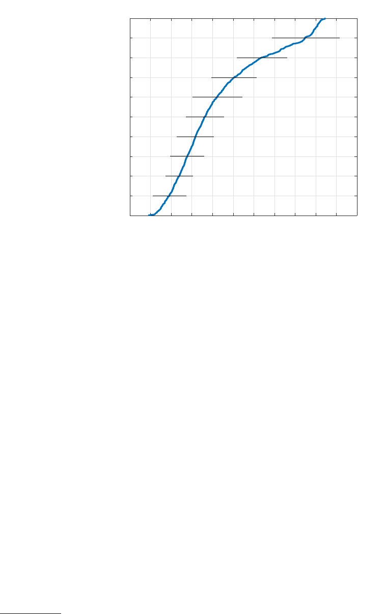
8 AARON BODOH-CREED, J
¨
ORN BOEHNKE, AND BRENT HICKMAN
0 2 4 6 8 10 12 14 16 18 20 22
Marginal Effect (Dollars)
0
0.1
0.2
0.3
0.4
0.5
0.6
0.7
0.8
0.9
1
CDF
At Least One Image in Description
Figure 7. Marginal Effect of Including at Least One Image in the Description
We require that the OLS estimator be asymptotically consistent as the size of the dataset grows.
If we were to collect more data, we could simultaneously define more leaves (increasing our ability
to detect heterogeneous marginal effects) and increase the size of the leaves (increasing the precision
of our OLS estimates). However, there is a tension between the size of the leaves and the amount
of heterogeneity we can detect. As we add more leaves to the tree, the regressor realizations within
each leaf will become more similar, and the decrease in regressor variability could make our OLS
estimates less precise. In the extreme, if we add leaves too quickly as our dataset grows, our OLS
models may not be consistent.
To solve this problem, we do not allow the trees to split on the variables we include in our
OLS regressions. Asymptotically, our trees will have an infinite set of data points at each leaf,
and the data in each leaf will be similar across the variables we allow the tree to use to define
splitting points. Since the regressors we include in the model at each leaf are not used to define
splitting points, there will be enough variation in those variables to accurately estimate the model
at each leaf. Each tree in our random forest provides a single estimate of the marginal effect of each
regressor at each data point (i.e., listing), so a random forest of 500 trees provides 500 estimates of
the marginal effect at each data point. We aggregate the estimates of the trees for each datum by
averaging the estimates of the trees.
We present our results in terms of cumulative density functions of the distribution of marginal
effects across the listings. Figure 7 displays the distribution of marginal effects of including an
image in a listing. We compute 95% confidence intervals for the marginal effects of the listings at
leaves created by the split. If the new leaf resulting from the merger is also empty, we recursively apply our algorithm
until a nonempty leaf is formed.
PREDICTING PRICE DISPERSION 9
-5 0 5 10 15 20 25
Marginal Effect (Dollars)
0
0.02
0.04
0.06
0.08
0.1
0.12
0.14
PDF
No Image in Description
Image in Description
Figure 8. Marginal Effect of Including at Least One Image in the Description
each decile by forming 1000 bootstrap samples of our estimation set and re-estimating the trees
with each bootstrap sample. We do not bootstrap the tree growing process. We provide confidence
bounds of the value realized for the listing at each decile of the distribution of marginal effects. We
do it this way because our later discussion will focus on differences between the marginal effects
at different quantile ranks of the distribution. To clarify, consider an alternative statistic that we
could have generated, but did not. We could have computed the CDF of the marginal effects for
each bootstrap run and then presented the 50
th
and 950
th
largest values at each decile. The listing
that occupied each quantile rank would vary between bootstrap runs. In addition, the standard
errors would appear deceptively small.
We estimate that 332 of our 1298 listings have marginal effects that are above the average at the
90% confidence level, while 592 of our listings have marginal effects that are significantly below the
average marginal effect at the 90% confidence level. In addition, the average marginal effect in the
first and ninth deciles are different from each other at the 99% confidence level.
We then divide our sample between the 216 listings that include at least one image in the
description and the 1082 listings that do not include such an image. The probability density
functions for the distribution of marginal effects of including more than one image for each group
are displayed in Figure 8. The average marginal effect for listings without an image in the description
is $8.06 and the average marginal effect for those that included an image in the description is $14.02,
a difference that is statistically significant at the 99% confidence level. The difference in means
implies that sellers are more likely to add a photo to a listing when the marginal effect on the price
is high, which is what one would expect of a profit-maximizing seller. From the distribution of
the marginal effects, it is clear that there are listings for which the marginal effect was under $5
and others for which the effect was over $15 under both distributions. In other words, the general
10 AARON BODOH-CREED, J
¨
ORN BOEHNKE, AND BRENT HICKMAN
0 0.5 1 1.5 2 2.5 3
Marginal Effect (Dollars)
0
0.1
0.2
0.3
0.4
0.5
0.6
0.7
0.8
0.9
1
CDF
Log Seller Score
Figure 9. Marginal Effect of Log Seller Score
patterns of the distribution of marginal effects obeys economic logic, but there are outliers in each
group.
Turning to the marginal effect of the seller score, there is a vast literature on the effectiveness
of eBay’s online reputation systems that leverages natural, field, and lab experiments. The early
literature assessed whether sellers earn a premium for a high reputation, implying that reputation
provides an incentive for good behavior (see Bajari and Horta¸csu 2004 [7] for a survey). The recent
literature has extended these analyses to directly studying whether reputation encourages good
behavior on the part of sellers (e.g., Cabral and Horta¸csu 2010 [18], Nosko and Tadelis 2015 [37]).
To the extent these papers conduct price regressions, typically the seller score enters the regression
either linearly or log-linearly, which eliminates the possibility of detecting heterogeneous marginal
effects
The cumulative distribution of the marginal effects of log seller score is displayed in Figure 9.
Obviously there is great deal of heterogeneity of the marginal effects of log seller score. 310 of
our listings have marginal effects above the mean at the 90% confidence level, while 502 of our
data points have marginal effects that are below the average at the 90% confidence level. The
distribution of the marginal effect of a one log-point change in seller score has a nontrivial support
with the lowest value just under $0.50 and the highest value just over $2.50.
One potential source of heterogeneity is that many aspects of the listing can serve as signals of a
seller’s professionalism. For example, a seller with a low reputation score and no item description
might benefit greatly from a marginal increase in his or her seller score. On the other hand, a seller
with a low reputation score that provides an elaborate listing with images and highly stylized text
that conveys a sense of professionalism might benefit less from an increase in her seller score since
PREDICTING PRICE DISPERSION 11
buyers already view the seller as a reliable professional. We tried a variety of different cuts of the
data to produce results similar in spirit to those displayed in Figure 8 for the number of images.
As it turns out, the distributions of marginal effects (for a one unit increase in reputation score)
appear roughly the same for “low score” and “high score” sellers under a variety of definitions of
these terms.

12 AARON BODOH-CREED, J
¨
ORN BOEHNKE, AND BRENT HICKMAN
Appendix D. Bag of Words
The full set of word stems we parsed from the text of each listing is described in the following
table along with the count of the number of listings in which the word appears. For clarity, the
table includes only one representative example of each word stem. It is important to note that the
following table pertains only to seller-customized content used as controls in our empirical analysis.
Stem Count Stem Count Stem Count
gb 1201 hour 199 good 146
new 1139 case 197 faster 145
black 978 game 197 b 141
box 662 feature 194 mail 140
brand 635 store 193 paypal 139
model 521 thank 187 return 137
latest 464 app 184 popular 136
ship 453 work 183 audio 133
free 389 power 180 inform 131
seal 382 original 179 system 131
all 373 processor 177 view 130
open 367 device 172 factory 124
include 361 special 168 service 124
screen 336 charger 167 experience 122
display 333 condition 165 look 122
have 324 support 164 facebook 121
no 303 read 161 additional 119
not 294 purchase 160 perfect 116
usb 265 receive 160 available 112
question 251 connect 158 warranty 111
offer 250 email 155 bid 110
only 243 internal 155 provide 110
more 231 charge 152 perform 109
package 220 million 151 sell 109
touch 212
payment 150 ad 108
fast 209 contact 149 full 106
battery 205 access 147 great 104
content 205 set 147 enjoy 99
cable 201 technology 147 detail 98

PREDICTING PRICE DISPERSION 13
Stem Count Stem Count Stem Count
require 98 cover 66 insure 38
accept 97 number 61 paid 37
test 97 delivery 60 leather 35
price 95 description 60 part 35
accessory 94 must 60 combine 34
best 94 except 58 receipt 34
state 94 love 58 fedex 33
custom 93 policy 58 friend 32
buyer 92 locate 56 info 30
fully 92 date 55 shipment 30
need 91
tax 55 describe 29
feedback 89 allow 54 change 28
note 89 position 54 damage 27
exchange 87 photo 53 separate 25
sale 87 refund 53 restock 24
start 85 top 52 process 23
check 84 identify 51 clean 22
actual 82 quickly 50 scratch 22
manufacturer 82 beautifully 49 concern 17
approximate 81 cost 48 fair 17
favorite 81 fee 48 credit 15
home 80 off 48 three 14
design 78 quality 44 win 13
well 77 sold 44 carefully 12
type 76 help 43 inspect 12
busy 75 close 42 discount 10
back 73 fluid 42 law 9
first 70 response 42 reserve 9
seller 70 treatment 41 wear 9
like 69 issue 40 invoice 8
pay 68 complete 39 appear 5
rate 68 immediate 39
left 67 guarante 38
